Spectroscopic Data Reduction

Spectroscopic data reduction is the process of converting raw spectroscopic images from a spectrograph into a calibrated spectrum. This process involves several steps, including bias subtraction, flat fielding, wavelength calibration, and extraction of the spectrum. In this notebook, we will go through the process of reducing a spectroscopic image using Python.

The CCD pre-processing steps are as usual: bias/dark subtraction, flat fielding, and cosmic ray removal. The spectroscopic data reduction steps are: extraction of the spectrum, wavelength calibration and flux calibration. Here we will focus mostly on the spectroscopic data reduction steps. After the data reduction, the spectrum can be used for scientific analysis, such as measuring redshifts, line identifications, and measuring line fluxes. In this notebook, we will reduce a 2D spectrum of an afterglow of a gamma-ray burst (GRB). Since this tutorial is prepared for the Project No. 5 of our TAO class, I leave the scientific analysis of the spectrum to readers.

The data used in this notebook is from the Subaru Telescope’s Faint Object Camera and Spectrograph (FOCAS). The data is 2D images of a spectrum of an afterglow of a GRB, GRB 130606A, which is a significantly redshifted source at \(z\sim5.9\). The data was taken on June 7, 2013, using the VPH900 grism, which covers the wavelength range of 7500-10450 Angstroms (Subaru FOCAS Hompage).

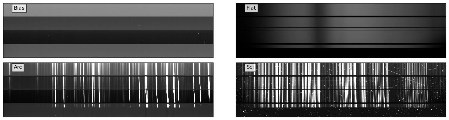
Let’s start by organizing the data and displaying the 2D spectral images.

import warnings
from pathlib import Path

import numpy as np
import plotly.express as px
import plotly.graph_objects as go
import plotly.io as pio
import preproc  # custom module for data reduction
from astropy import units as u
from astropy.io import fits
from astropy.modeling.fitting import LevMarLSQFitter
from astropy.modeling.models import Chebyshev2D
from astropy.nddata import CCDData
from astropy.stats import gaussian_fwhm_to_sigma, sigma_clip
from astropy.table import Table
from astropy.visualization import ZScaleInterval
from ccdproc import combine, cosmicray_lacosmic, gain_correct
from matplotlib import pyplot as plt
from mpl_toolkits.axes_grid1 import make_axes_locatable
from numpy.polynomial.chebyshev import chebfit, chebval
from rascal import util
from rascal.atlas import Atlas
from rascal.calibrator import Calibrator
from scipy.ndimage import map_coordinates, median_filter
from scipy.signal import peak_widths
from skimage.feature import peak_local_max
from specutils import Spectrum1D
from specutils.manipulation import FluxConservingResampler

pio.renderers.default = "notebook"

# plt.rcParams['axes.linewidth'] = 2
plt.rcParams["font.size"] = 12
plt.rcParams["axes.labelsize"] = 14

WD = Path("./data/proj5")
RAWDIR = WD / "raw" / "P03hbahk0304145443GZ_data"
OUTDIR = WD / "out"

if not OUTDIR.exists():
    OUTDIR.mkdir(parents=True)

warnings.filterwarnings("ignore", category=UserWarning, append=True)

/opt/anaconda3/envs/main/lib/python3.11/site-packages/rascal/calibrator.py:9: TqdmExperimentalWarning:

Using `tqdm.autonotebook.tqdm` in notebook mode. Use `tqdm.tqdm` instead to force console mode (e.g. in jupyter console)

def make_summary_table_focas(rawdir, suffix=".fits.gz"):
    """Make a summary table of the raw data in the directory. This function is
    specifically designed for the data taken with the FOCAS instrument.

    Args:
        rawdir (pathlib.Path): The directory containing the raw data.
        suffix (str, optional): The suffix of the raw data files. Defaults to
            '.fits.gz'.

    Returns:
        stab (astropy.table.Table): The summary table of the raw data in the directory.

    """
    # making a summary table
    summary = []
    for f in rawdir.glob("*" + suffix):
        hdr = fits.getheader(f)

        # getting the filter information from the header
        filt1 = hdr["FILTER01"]
        filt2 = hdr["FILTER02"]
        filt3 = hdr["FILTER03"]

        X = hdr["AIRMASS"]  # airmass
        disp = hdr["DISPERSR"]  # disperser

        # appending the data to the summary list
        summary.append(
            [
                f.name,
                hdr["DATE-OBS"],
                hdr["OBJECT"],
                hdr["RA"],
                hdr["DEC"],
                hdr["DATA-TYP"],
                hdr["EXPTIME"],
                X,
                hdr["ALTITUDE"],
                disp,
                hdr["SLT-WID"],
                hdr["SLT-PA"],
                hdr["SLIT"],
                filt1,
                filt2,
                filt3,
                hdr["UT-STR"],
                hdr["UT-END"],
            ]
        )

    # creating the summary table
    stab = Table(
        rows=summary,
        names=[
            "filename",
            "date-obs",
            "object",
            "ra",
            "dec",
            "type",
            "exptime",
            "airmass",
            "altitude",
            "disperser",
            "slit-width",
            "slit-pa",
            "slit",
            "filter1",
            "filter2",
            "filter3",
            "ut-str",
            "ut-end",
        ],
        dtype=[
            "U50",
            "U50",
            "U50",
            "U50",
            "U50",
            "U50",
            "f8",
            "f8",
            "f8",
            "U50",
            "f8",
            "f8",
            "U50",
            "U50",
            "U50",
            "U50",
            "U50",
            "U50",
        ],
    )
    return stab

summary_table = make_summary_table_focas(RAWDIR)
summary_table

Table length=60

filename	date-obs	object	ra	dec	type	exptime	airmass	altitude	disperser	slit-width	slit-pa	slit	filter1	filter2	filter3	ut-str	ut-end
str50	str50	str50	str50	str50	str50	float64	float64	float64	str50	float64	float64	str50	str50	str50	str50	str50	str50
FCSA00141794.fits.gz	2013-06-07	DOMEFLAT	11:17:48.038	+19:54:08.26	DOMEFLAT	3.0	1.0	89.9361	SCFCGRHD90	0.5	-90.3	SCFCSLLC08	NONE	SCFCFLSO58	NONE	04:37:11.906	04:37:15.139
FCSA00141920.fits.gz	2013-06-07	GRB 130606A	16:37:41.157	+29:47:45.71	OBJECT	1200.0	1.136	61.6129	SCFCGRHD90	0.5	-90.3	SCFCSLLC08	NONE	SCFCFLSO58	NONE	07:59:00.676	08:19:01.117
FCSA00141930.fits.gz	2013-06-07	GRB 130606A	16:37:41.230	+29:47:45.13	OBJECT	1200.0	1.038	74.4191	SCFCGRHD90	0.5	-90.3	SCFCSLLC08	NONE	SCFCFLSO58	NONE	09:03:28.980	09:23:29.405
FCSA00141848.fits.gz	2013-06-07	BIAS	11:39:50.841	+19:54:11.18	BIAS	0.0	1.0	89.9361	SCFCGRMR01	0.5	-90.3	SCFCSLLC20	NONE	SCFCFLSO58	NONE	04:59:10.571	04:59:10.574
FCSA00141916.fits.gz	2013-06-07	GRB 130606A	16:37:41.020	+29:47:44.75	OBJECT	1200.0	1.254	52.8249	SCFCGRHD90	0.5	-90.3	SCFCSLLC08	NONE	SCFCFLSO58	NONE	07:18:00.165	07:38:00.608
FCSA00141734.fits.gz	2013-06-06	BIAS	21:41:03.767	+17:46:28.41	BIAS	0.0	1.001	86.8997	SCFCGRHD90	0.5	-0.3	SCFCSLLC20	NONE	SCFCFLSO58	NONE	14:53:03.807	14:53:03.810
FCSA00141566.fits.gz	2013-06-06	DOMEFLAT	11:23:03.374	+19:54:09.25	DOMEFLAT	1.1	1.0	89.9625	SCFCGRHD90	0.5	-90.3	SCFCSLLC20	NONE	SCFCFLSO58	NONE	04:46:28.971	04:46:30.721
FCSA00141576.fits.gz	2013-06-06	DOMEFLAT	11:26:18.779	+19:54:09.76	DOMEFLAT	3.0	1.0	89.9625	SCFCGRHD90	0.5	-90.3	SCFCSLLC08	NONE	SCFCFLSO58	NONE	04:49:43.639	04:49:46.993
FCSA00141822.fits.gz	2013-06-07	DOMEFLAT	11:26:05.681	+19:54:09.65	DOMEFLAT	1.1	1.0	89.9361	SCFCGRHD90	0.5	-90.3	SCFCSLLC20	NONE	SCFCFLSO58	NONE	04:45:27.990	04:45:29.664
...	...	...	...	...	...	...	...	...	...	...	...	...	...	...	...	...	...
FCSA00141730.fits.gz	2013-06-06	BIAS	23:03:44.623	-01:20:01.29	BIAS	0.0	1.169	58.8068	SCFCGRHD90	0.5	-0.3	SCFCSLLC20	NONE	SCFCFLSO58	NONE	14:52:13.406	14:52:13.410
FCSA00141818.fits.gz	2013-06-07	DOMEFLAT	11:25:08.002	+19:54:09.51	DOMEFLAT	1.1	1.0	89.9361	SCFCGRHD90	0.5	-90.3	SCFCSLLC20	NONE	SCFCFLSO58	NONE	04:44:30.393	04:44:31.697
FCSA00142010.fits.gz	2013-06-07	Feige110	23:20:01.964	-05:10:51.68	OBJECT	120.0	1.208	55.8712	SCFCGRHD90	0.5	-405.3	SCFCSLLC20	NONE	SCFCFLSO58	NONE	15:03:10.694	15:05:11.030
FCSA00141798.fits.gz	2013-06-07	DOMEFLAT	11:18:59.560	+19:54:08.48	DOMEFLAT	3.0	1.0	89.9361	SCFCGRHD90	0.5	-90.3	SCFCSLLC08	NONE	SCFCFLSO58	NONE	04:38:23.184	04:38:26.574
FCSA00141854.fits.gz	2013-06-07	BIAS	11:41:06.075	+19:54:11.27	BIAS	0.0	1.0	89.9361	SCFCGRMR01	0.5	-90.3	SCFCSLLC20	NONE	SCFCFLSO58	NONE	05:00:25.637	05:00:25.674
FCSA00141586.fits.gz	2013-06-06	BIAS	11:32:20.002	+19:54:10.54	BIAS	0.0	1.0	89.9625	SCFCGRHD90	0.5	-90.3	SCFCSLLC20	NONE	SCFCFLSO58	NONE	04:55:43.880	04:55:43.883
FCSA00141562.fits.gz	2013-06-06	DOMEFLAT	11:22:06.397	+19:54:09.10	DOMEFLAT	1.1	1.0	89.9625	SCFCGRHD90	0.5	-90.3	SCFCSLLC20	NONE	SCFCFLSO58	NONE	04:45:32.080	04:45:33.717
FCSA00141572.fits.gz	2013-06-06	DOMEFLAT	11:25:16.188	+19:54:09.60	DOMEFLAT	3.0	1.0	89.9625	SCFCGRHD90	0.5	-90.3	SCFCSLLC08	NONE	SCFCFLSO58	NONE	04:48:41.382	04:48:44.710
FCSA00141728.fits.gz	2013-06-06	BIAS	23:19:58.381	-05:11:14.89	BIAS	0.0	1.248	53.1982	SCFCGRHD90	0.5	-0.3	SCFCSLLC20	NONE	SCFCFLSO58	NONE	14:51:48.193	14:51:48.197
FCSA00141800.fits.gz	2013-06-07	DOMEFLAT	11:19:30.656	+19:54:08.58	DOMEFLAT	3.0	1.0	89.9361	SCFCGRHD90	0.5	-90.3	SCFCSLLC08	NONE	SCFCFLSO58	NONE	04:38:54.202	04:38:57.612

biastab = summary_table[summary_table["type"] == "BIAS"]
flattab = summary_table[summary_table["type"] == "DOMEFLAT"]
arctab = summary_table[
    (summary_table["type"] == "COMPARISON") & (summary_table["slit"] == "SCFCSLLC08")
]
scitab = summary_table[summary_table["object"] == "GRB 130606A"]
stdtab_f110 = summary_table[
    (summary_table["object"] == "Feige110") & (summary_table["type"] == "OBJECT")
]
stdtab_f34 = summary_table[
    (summary_table["object"] == "Feige34") & (summary_table["type"] == "OBJECT")
]

# for displaying in zscale
interval = ZScaleInterval()

# plotting the images
fig, axes = plt.subplots(2, 2, figsize=(15, 4))
titles = ["Bias", "Flat", "Arc", "Sci"]
bias = fits.getdata(RAWDIR / biastab["filename"][0])
flat = fits.getdata(RAWDIR / flattab["filename"][0])
arc = fits.getdata(RAWDIR / arctab["filename"][0])
sci = fits.getdata(RAWDIR / scitab["filename"][0])
for i, img in enumerate([bias, flat, arc, sci]):
    vmin, vmax = interval.get_limits(img)
    ax = axes[i // 2][i % 2]
    ax.imshow(img.T, cmap="gray", origin="lower", vmin=vmin, vmax=vmax)
    ax.text(
        0.05,
        0.95,
        titles[i],
        transform=ax.transAxes,
        ha="left",
        va="top",
        bbox=dict(facecolor="white", alpha=0.8),
    )
    ax.tick_params(axis="both", length=0.0, labelleft=False, labelbottom=False)
plt.tight_layout()

del bias, flat, arc, sci

Preprocessing of the Raw Images

Preprocessing of the raw images is the first step in the data reduction process. The raw images are usually not ready for scientific analysis and need to be preprocessed before they can be used for scientific analysis. The preprocessing steps include the following:

1. Bias subtraction

2. Dark subtraction

3. Flat fielding

4. Cosmic ray removal

There are lots of software available for preprocessing the raw images. In this tutorial, we will use the ccdproc package for preprocessing the raw images. The ccdproc package is a Python package for reducing astronomical data taken with CCD cameras. It provides many of the necessary tools for processing of CCD images. For more information on the ccdproc package, please visit the documentation, and for the complete guide on the reduction process for astronomical images using Python, CCD Reduction and Photometry Guide.

In this notebook, we will preprocess the raw images using preproc.py script. This script is available in the tutorial directory. Dark subtraction will not be performed in this notebook since the amount of dark current in the images is negligible.

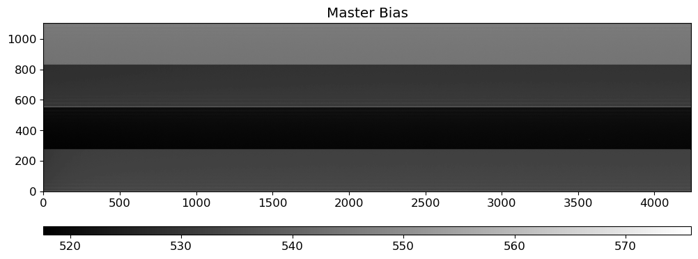
Making the Master Bias

Before making the master bias, we need to check the bias images for any defects. We skip this step here, but it is important to check since the bias images are used to calibrate all the other images. If there are defects in the bias images, they will be propagated to all the other images.

The master bias is made by combining all the bias images. The master bias will be subtracted from all the images to remove the bias level. For combining the bias images, the sigma-clipping algorithm is used to reject outliers and then the average of the remaining images is calculated.

biaslist = [RAWDIR / f for f in biastab["filename"]]
_ = preproc.combine_bias(biaslist, outdir=OUTDIR, outname="MBias.fits")
del _

Show code cell output Hide code cell output

INFO: using the unit adu passed to the FITS reader instead of the unit adu in the FITS file. [astropy.nddata.ccddata]
INFO: An exception happened while extracting WCS information from the Header.
InconsistentAxisTypesError: ERROR 4 in wcs_types() at line 3140 of file cextern/wcslib/C/wcs.c:
Unmatched celestial axes.
 [astropy.nddata.ccddata]
INFO: using the unit adu passed to the FITS reader instead of the unit adu in the FITS file. [astropy.nddata.ccddata]
INFO: An exception happened while extracting WCS information from the Header.
InconsistentAxisTypesError: ERROR 4 in wcs_types() at line 3140 of file cextern/wcslib/C/wcs.c:
Unmatched celestial axes.
 [astropy.nddata.ccddata]
INFO: using the unit adu passed to the FITS reader instead of the unit adu in the FITS file. [astropy.nddata.ccddata]
INFO: An exception happened while extracting WCS information from the Header.
InconsistentAxisTypesError: ERROR 4 in wcs_types() at line 3140 of file cextern/wcslib/C/wcs.c:
Unmatched celestial axes.
 [astropy.nddata.ccddata]

WARNING: FITSFixedWarning: PC001001= 1.00000000 / Pixel Coordinate translation matrix 
this form of the PCi_ja keyword is deprecated, use PCi_ja. [astropy.wcs.wcs]
WARNING: FITSFixedWarning: PC001002= 0.00000000 / Pixel Coordinate translation matrix 
this form of the PCi_ja keyword is deprecated, use PCi_ja. [astropy.wcs.wcs]
WARNING: FITSFixedWarning: PC002001= 0.00000000 / Pixel Coordinate translation matrix 
this form of the PCi_ja keyword is deprecated, use PCi_ja. [astropy.wcs.wcs]
WARNING: FITSFixedWarning: PC002002= 1.00000000 / Pixel Coordinate translation matrix 
this form of the PCi_ja keyword is deprecated, use PCi_ja. [astropy.wcs.wcs]
WARNING: FITSFixedWarning: RADECSYS= 'FK5 ' / The equatorial coordinate system 
the RADECSYS keyword is deprecated, use RADESYSa. [astropy.wcs.wcs]
WARNING: FITSFixedWarning: 'datfix' made the change 'Set MJD-OBS to 56450.000000 from DATE-OBS.
Set DATE-END to '2013-06-07T04:59:10.645' from MJD-END'. [astropy.wcs.wcs]
WARNING: FITSFixedWarning: 'unitfix' made the change 'Changed units:
  'degree' -> 'deg'. [astropy.wcs.wcs]
WARNING: FITSFixedWarning: 'celfix' made the change 'Unmatched celestial axes'. [astropy.wcs.wcs]
WARNING: FITSFixedWarning: 'datfix' made the change 'Set MJD-OBS to 56449.000000 from DATE-OBS.
Set DATE-END to '2013-06-06T14:53:03.880' from MJD-END'. [astropy.wcs.wcs]
WARNING: FITSFixedWarning: 'datfix' made the change 'Set MJD-OBS to 56449.000000 from DATE-OBS.
Set DATE-END to '2013-06-06T04:56:58.652' from MJD-END'. [astropy.wcs.wcs]

INFO: using the unit adu passed to the FITS reader instead of the unit adu in the FITS file. [astropy.nddata.ccddata]
INFO: An exception happened while extracting WCS information from the Header.
InconsistentAxisTypesError: ERROR 4 in wcs_types() at line 3140 of file cextern/wcslib/C/wcs.c:
Unmatched celestial axes.
 [astropy.nddata.ccddata]
INFO: using the unit adu passed to the FITS reader instead of the unit adu in the FITS file. [astropy.nddata.ccddata]
INFO: An exception happened while extracting WCS information from the Header.
InconsistentAxisTypesError: ERROR 4 in wcs_types() at line 3140 of file cextern/wcslib/C/wcs.c:
Unmatched celestial axes.
 [astropy.nddata.ccddata]
INFO: using the unit adu passed to the FITS reader instead of the unit adu in the FITS file. [astropy.nddata.ccddata]
INFO: An exception happened while extracting WCS information from the Header.
InconsistentAxisTypesError: ERROR 4 in wcs_types() at line 3140 of file cextern/wcslib/C/wcs.c:
Unmatched celestial axes.
 [astropy.nddata.ccddata]

WARNING: FITSFixedWarning: 'datfix' made the change 'Set MJD-OBS to 56450.000000 from DATE-OBS.
Set DATE-END to '2013-06-07T04:59:35.780' from MJD-END'. [astropy.wcs.wcs]
WARNING: FITSFixedWarning: 'datfix' made the change 'Set MJD-OBS to 56450.000000 from DATE-OBS.
Set DATE-END to '2013-06-07T15:06:35.545' from MJD-END'. [astropy.wcs.wcs]
WARNING: FITSFixedWarning: 'datfix' made the change 'Set MJD-OBS to 56450.000000 from DATE-OBS.
Set DATE-END to '2013-06-07T05:00:00.751' from MJD-END'. [astropy.wcs.wcs]

INFO: using the unit adu passed to the FITS reader instead of the unit adu in the FITS file. [astropy.nddata.ccddata]
INFO: An exception happened while extracting WCS information from the Header.
InconsistentAxisTypesError: ERROR 4 in wcs_types() at line 3140 of file cextern/wcslib/C/wcs.c:
Unmatched celestial axes.
 [astropy.nddata.ccddata]
INFO: using the unit adu passed to the FITS reader instead of the unit adu in the FITS file. [astropy.nddata.ccddata]
INFO: An exception happened while extracting WCS information from the Header.
InconsistentAxisTypesError: ERROR 4 in wcs_types() at line 3140 of file cextern/wcslib/C/wcs.c:
Unmatched celestial axes.
 [astropy.nddata.ccddata]
INFO: using the unit adu passed to the FITS reader instead of the unit adu in the FITS file. [astropy.nddata.ccddata]
INFO: An exception happened while extracting WCS information from the Header.
InconsistentAxisTypesError: ERROR 4 in wcs_types() at line 3140 of file cextern/wcslib/C/wcs.c:
Unmatched celestial axes.
 [astropy.nddata.ccddata]

WARNING: FITSFixedWarning: 'datfix' made the change 'Set MJD-OBS to 56449.000000 from DATE-OBS.
Set DATE-END to '2013-06-06T04:56:34.054' from MJD-END'. [astropy.wcs.wcs]
WARNING: FITSFixedWarning: 'datfix' made the change 'Set MJD-OBS to 56450.000000 from DATE-OBS.
Set DATE-END to '2013-06-07T15:07:00.686' from MJD-END'. [astropy.wcs.wcs]
WARNING: FITSFixedWarning: 'datfix' made the change 'Set MJD-OBS to 56450.000000 from DATE-OBS.
Set DATE-END to '2013-06-07T15:07:53.456' from MJD-END'. [astropy.wcs.wcs]

INFO: using the unit adu passed to the FITS reader instead of the unit adu in the FITS file. [astropy.nddata.ccddata]
INFO: An exception happened while extracting WCS information from the Header.
InconsistentAxisTypesError: ERROR 4 in wcs_types() at line 3140 of file cextern/wcslib/C/wcs.c:
Unmatched celestial axes.
 [astropy.nddata.ccddata]
INFO: using the unit adu passed to the FITS reader instead of the unit adu in the FITS file. [astropy.nddata.ccddata]
INFO: An exception happened while extracting WCS information from the Header.
InconsistentAxisTypesError: ERROR 4 in wcs_types() at line 3140 of file cextern/wcslib/C/wcs.c:
Unmatched celestial axes.
 [astropy.nddata.ccddata]
INFO: using the unit adu passed to the FITS reader instead of the unit adu in the FITS file. [astropy.nddata.ccddata]
INFO: An exception happened while extracting WCS information from the Header.
InconsistentAxisTypesError: ERROR 4 in wcs_types() at line 3140 of file cextern/wcslib/C/wcs.c:
Unmatched celestial axes.
 [astropy.nddata.ccddata]

WARNING: FITSFixedWarning: 'datfix' made the change 'Set MJD-OBS to 56449.000000 from DATE-OBS.
Set DATE-END to '2013-06-06T04:56:09.042' from MJD-END'. [astropy.wcs.wcs]
WARNING: FITSFixedWarning: 'datfix' made the change 'Set MJD-OBS to 56449.000000 from DATE-OBS.
Set DATE-END to '2013-06-06T14:53:29.035' from MJD-END'. [astropy.wcs.wcs]
WARNING: FITSFixedWarning: 'datfix' made the change 'Set MJD-OBS to 56450.000000 from DATE-OBS.
Set DATE-END to '2013-06-07T15:06:10.558' from MJD-END'. [astropy.wcs.wcs]

INFO: using the unit adu passed to the FITS reader instead of the unit adu in the FITS file. [astropy.nddata.ccddata]
INFO: An exception happened while extracting WCS information from the Header.
InconsistentAxisTypesError: ERROR 4 in wcs_types() at line 3140 of file cextern/wcslib/C/wcs.c:
Unmatched celestial axes.
 [astropy.nddata.ccddata]
INFO: using the unit adu passed to the FITS reader instead of the unit adu in the FITS file. [astropy.nddata.ccddata]
INFO: An exception happened while extracting WCS information from the Header.
InconsistentAxisTypesError: ERROR 4 in wcs_types() at line 3140 of file cextern/wcslib/C/wcs.c:
Unmatched celestial axes.
 [astropy.nddata.ccddata]
INFO: using the unit adu passed to the FITS reader instead of the unit adu in the FITS file. [astropy.nddata.ccddata]
INFO: An exception happened while extracting WCS information from the Header.
InconsistentAxisTypesError: ERROR 4 in wcs_types() at line 3140 of file cextern/wcslib/C/wcs.c:
Unmatched celestial axes.
 [astropy.nddata.ccddata]

WARNING: FITSFixedWarning: 'datfix' made the change 'Set MJD-OBS to 56449.000000 from DATE-OBS.
Set DATE-END to '2013-06-06T04:55:19.314' from MJD-END'. [astropy.wcs.wcs]
WARNING: FITSFixedWarning: 'datfix' made the change 'Set MJD-OBS to 56450.000000 from DATE-OBS.
Set DATE-END to '2013-06-07T04:58:45.726' from MJD-END'. [astropy.wcs.wcs]
WARNING: FITSFixedWarning: 'datfix' made the change 'Set MJD-OBS to 56449.000000 from DATE-OBS.
Set DATE-END to '2013-06-06T14:52:38.925' from MJD-END'. [astropy.wcs.wcs]

INFO: using the unit adu passed to the FITS reader instead of the unit adu in the FITS file. [astropy.nddata.ccddata]
INFO: An exception happened while extracting WCS information from the Header.
InconsistentAxisTypesError: ERROR 4 in wcs_types() at line 3140 of file cextern/wcslib/C/wcs.c:
Unmatched celestial axes.
 [astropy.nddata.ccddata]
INFO: using the unit adu passed to the FITS reader instead of the unit adu in the FITS file. [astropy.nddata.ccddata]
INFO: An exception happened while extracting WCS information from the Header.
InconsistentAxisTypesError: ERROR 4 in wcs_types() at line 3140 of file cextern/wcslib/C/wcs.c:
Unmatched celestial axes.
 [astropy.nddata.ccddata]
INFO: using the unit adu passed to the FITS reader instead of the unit adu in the FITS file. [astropy.nddata.ccddata]
INFO: An exception happened while extracting WCS information from the Header.
InconsistentAxisTypesError: ERROR 4 in wcs_types() at line 3140 of file cextern/wcslib/C/wcs.c:
Unmatched celestial axes.
 [astropy.nddata.ccddata]

WARNING: FITSFixedWarning: 'datfix' made the change 'Set MJD-OBS to 56450.000000 from DATE-OBS.
Set DATE-END to '2013-06-07T15:07:26.756' from MJD-END'. [astropy.wcs.wcs]
WARNING: FITSFixedWarning: 'datfix' made the change 'Set MJD-OBS to 56449.000000 from DATE-OBS.
Set DATE-END to '2013-06-06T14:52:13.481' from MJD-END'. [astropy.wcs.wcs]
WARNING: FITSFixedWarning: 'datfix' made the change 'Set MJD-OBS to 56450.000000 from DATE-OBS.
Set DATE-END to '2013-06-07T05:00:25.744' from MJD-END'. [astropy.wcs.wcs]

INFO: using the unit adu passed to the FITS reader instead of the unit adu in the FITS file. [astropy.nddata.ccddata]
INFO: An exception happened while extracting WCS information from the Header.
InconsistentAxisTypesError: ERROR 4 in wcs_types() at line 3140 of file cextern/wcslib/C/wcs.c:
Unmatched celestial axes.
 [astropy.nddata.ccddata]
INFO: using the unit adu passed to the FITS reader instead of the unit adu in the FITS file. [astropy.nddata.ccddata]
INFO: An exception happened while extracting WCS information from the Header.
InconsistentAxisTypesError: ERROR 4 in wcs_types() at line 3140 of file cextern/wcslib/C/wcs.c:
Unmatched celestial axes.
 [astropy.nddata.ccddata]

WARNING: FITSFixedWarning: 'datfix' made the change 'Set MJD-OBS to 56449.000000 from DATE-OBS.
Set DATE-END to '2013-06-06T04:55:43.954' from MJD-END'. [astropy.wcs.wcs]
WARNING: FITSFixedWarning: 'datfix' made the change 'Set MJD-OBS to 56449.000000 from DATE-OBS.
Set DATE-END to '2013-06-06T14:51:48.267' from MJD-END'. [astropy.wcs.wcs]

mbias = OUTDIR / "MBias.fits"
mbias_img = fits.getdata(mbias)
fig = plt.figure(figsize=(12, 6))
ax = fig.add_subplot(111)
vmin, vmax = interval.get_limits(mbias_img)
im = ax.imshow(mbias_img.T, cmap="gray", origin="lower", vmin=vmin, vmax=vmax)
ax.set_title("Master Bias")
divider = make_axes_locatable(ax)
cax = divider.append_axes("bottom", size="5%", pad=0.5)
plt.colorbar(im, cax=cax, orientation="horizontal")
fig.show()

Making Master Flat

Not like the photometric observation, spectroscopic flat image is typically taken with something like halogen lamp or tungsten lamp, which is inevitably not uniform especially for the dispersion direction. Therefore, we need to make a master flat image flat, which involves modeling the flat spectrum and dividing the flat image by the model. To obtain a good master flat, we need to:

1. Examine the flat spectra: do they show any variablity throughout the observation? can we combine them without any further consideration? do they have any features like wiggles or bumps? do they have any discontinuity?

2. Model the flat spectra: we can use a polynomial (or smoothing convolution) to model the flat spectrum. The degree of the polynomial (or size of the smoothing kernel) should be determined by the complexity of the flat spectrum.

3. Normalize the flat spectra: divide the flat image by the model to obtain a normalized flat image.

Combining can be done either before or after the modeling. If the flat spectra are stable, we can combine them first and then model the combined flat spectrum. If the flat spectra are not stable, we can model each flat spectrum and then combine the normalized flat images. If the flat spectra show significant variability, we can also consider not combining them at all.

Because of this complexity, making a master flat can be a time-consuming part of the data reduction process. Moreover, the quality of the master flat directly affects the quality of the reduced science images, which may introduce systematic errors if not done properly. Therefore, the spectroscopic flat fielding is often omitted in the data reduction process, when the flat fielding conversely introduces more errors than it corrects.

Checking for Flat Image Shift

The flat image may shift slightly depending on the telescope’s pointing direction. Since different images might require different flats, it can be risky to median combine all the flat images taken overnight. We should perform a quick and rough check to see if there is a shift in the flat images.

To avoid bias might arise from this shift, it is recommended to take flat images at the same pointing direction as the science images. However, if the shift is small, we can still use the median combined flat image for calibration.

Note

With the same reason, we should be careful when we reduce the arc frames. The location of the lines in the arc spectrum may shift slightly depending on the telescope’s pointing direction. Therefore, it is strongly recommended to take arc frames at the same pointing direction as the science frames.

We should check for the shift in the arc frames, but we will skip this process for simplicity.

However, unlike the flat fielding, the wavelength calibration is of critical importance in the spectroscopic data reduction process, since few percent of errors in the wavelength calibration can introduce systematic errors in the scientific analysis, such as the measurement of the redshift of galaxies. Therefore, we should always check for the shift in the arc frames before wavelength calibration.

In this notebook, we will skip this process for simplicity, but you should always check for flat image shift in your own data. We will assume that the flat images are already aligned, and we will proceed to combine them.

flattab_exp3 = flattab[flattab["exptime"] == 3.0]
flattab_exp1 = flattab[flattab["exptime"] == 1.1]
flatlist_exp3 = [RAWDIR / f for f in flattab_exp3["filename"]]
flatlist_exp1 = [RAWDIR / f for f in flattab_exp1["filename"]]

mbias = OUTDIR / "MBias.fits"
_ = preproc.make_master_flat(
    flatlist_exp3,
    outdir=OUTDIR,
    outname="MFlat03.0.fits",
    mbias=mbias,
    filter_key="FILTER02",
    verbose=False,
)
_ = preproc.make_master_flat(
    flatlist_exp1,
    outdir=OUTDIR,
    outname="MFlat01.1.fits",
    mbias=mbias,
    filter_key="FILTER02",
    verbose=False,
)
del _

Comparing with the Standard Star Profile

Typical flat spectra shows many wiggles and bumps. Yet, we don’t know if these features are originated from the grating (as a representation of common instruments that can affect the both flat and science frames), which in turn will affect our science frame equally. If they are not due to the grating, such as filters in front of the flat-field lamp, the extreme difference in color temperature between the lamps and the object of interest, or wavelength-dependent variations in the reflectivity of the paint used for the flat-field screen (Massey & Hansen, 2010), they are not going to present on the science frame.

Let’s see if a supposedly smooth source (in this case, a standard star) has same “wiggles” and “bumps” on its spectrum. If this is the case, we should normalize the flat spectrum with a constant value (or a “low-order” functional model). If not, we should adopt “high-order” model or constant to normalize our flat field. For more information, please refer to Section 3.1., Massey & Hansen (2010).

fig = plt.figure(figsize=(12, 6))
ax = fig.add_subplot(111)
flat03 = fits.getdata(OUTDIR / "MFlat03.0.fits")
vmin, vmax = interval.get_limits(flat03)
im = ax.imshow(flat03.T, cmap="gray", origin="lower", vmin=vmin, vmax=vmax)
ax.set_title("Master Flat (3.0s)")

fig = plt.figure(figsize=(12, 6))
ax = fig.add_subplot(111)
flat01 = fits.getdata(OUTDIR / "MFlat01.1.fits")
vmin, vmax = interval.get_limits(flat01)
im = ax.imshow(flat03.T, cmap="gray", origin="lower", vmin=vmin, vmax=vmax)
ax.set_title("Master Flat (1.1s)")

fig = plt.figure(figsize=(12, 6))
ax = fig.add_subplot(111)
f34 = fits.getdata(RAWDIR / stdtab_f34["filename"][0])
vmin, vmax = interval.get_limits(f34)
im = ax.imshow(f34.T, cmap="gray", origin="lower", vmin=vmin, vmax=vmax)
ax.set_title("Feige34 (Standard Star)")

Text(0.5, 1.0, 'Feige34 (Standard Star)')

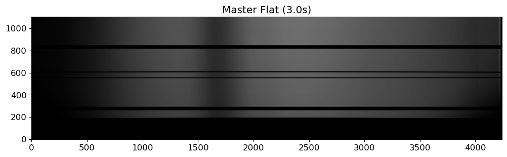
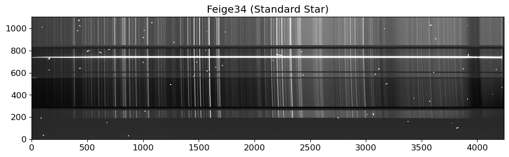
fig = plt.figure(figsize=(12, 6))
ax = fig.add_subplot(211)
ax.plot(flat03[:, 700])
ax.text(
    0.05,
    0.95,
    "Master Flat, 3.0s, Row 700",
    transform=ax.transAxes,
    ha="left",
    va="top",
)
ax.grid()
ax = fig.add_subplot(212)
ax.plot(f34[:, 737])
ax.text(
    0.05, 0.95, "Feige34, Row 700, Raw", transform=ax.transAxes, ha="left", va="top"
)
ax.grid()

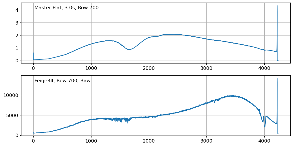
Although we can see some tiny wiggles in the flat spectrum, this is not significant enough to adopt higher-order polynomials to model the flat spectrum, as opposed to the case if we have significant fringe patterns. If you closely examine the flat spectrum, you will see that the wiggles are not random, but rather located at the atmospheric absorption lines. This is because the flat image is taken with a lamp, and the lamp light is absorbed by the atmosphere at these absorption lines. Since the absorption lines are not random, we can safely ignore them when modeling the flat spectrum.

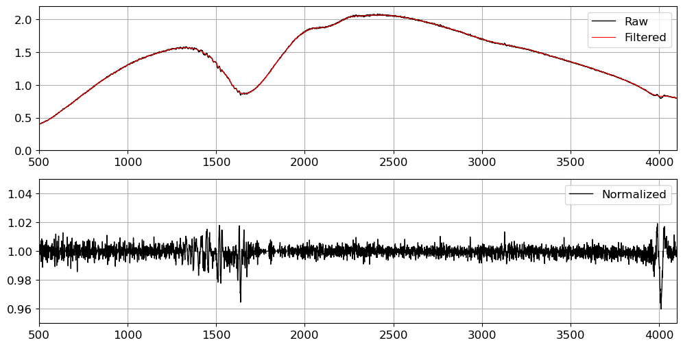
Here we model the flat spectrum with median filtering, which is a simple and effective way to remove noise while preserving the shape of the spectrum. We will use a median filter in the dispersion direction to model the flat spectrum, with a window size of 100 pixels. This is a good starting point, but you may need to adjust the window size depending on the complexity of the flat spectrum.

Note

Although I compared the horizontal profile of the standard star and the flat image for convenience, it might as well natural to compare the final extracted spectra of the standard star after applying both the high-order and low-order model of the flat field.

For simplicity, we will only use the combined flat image taken with the exposure time of 3 seconds. In practice, you may use all the flat images taken with different exposure times to make a master flat, or you can use the flat images taken with long and short exposure times to make a bad pixel map.

# median filtering the flat field image along the dispersion axis
flat03_filt = median_filter(flat03, size=50, axes=0)
# normalizing the flat field image
normflat = flat03 / flat03_filt

fig = plt.figure(figsize=(12, 6))
ax = fig.add_subplot(211)
ax.plot(flat03[:, 700], c="k", label="Raw", lw=1)
ax.plot(flat03_filt[:, 700], c="r", label="Filtered", lw=0.8)
ax.set_xlim(500, 4100)
ax.set_ylim(0, 2.2)
ax.legend()
ax.grid()
ax = fig.add_subplot(212)
ax.plot(normflat[:, 700], c="k", label="Normalized", lw=1)
ax.set_xlim(500, 4100)
ax.set_ylim(0.95, 1.05)
ax.legend()
ax.grid()

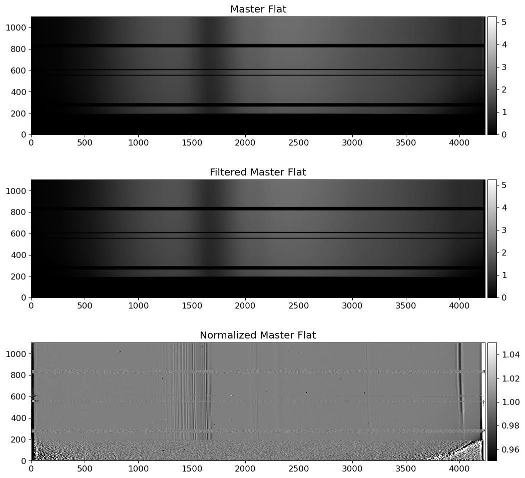
fig = plt.figure(figsize=(12, 12))
ax = fig.add_subplot(311)
vmin, vmax = interval.get_limits(flat03)
im = ax.imshow(flat03.T, cmap="gray", origin="lower", vmin=vmin, vmax=vmax)
ax.set_title("Master Flat")
divider = make_axes_locatable(ax)
cax = divider.append_axes("right", size="2%", pad=0.05)
plt.colorbar(im, cax=cax)
ax = fig.add_subplot(312)
im = ax.imshow(flat03_filt.T, cmap="gray", origin="lower", vmin=vmin, vmax=vmax)
ax.set_title("Filtered Master Flat")
divider = make_axes_locatable(ax)
cax = divider.append_axes("right", size="2%", pad=0.05)
plt.colorbar(im, cax=cax)
ax = fig.add_subplot(313)
vmin, vmax = interval.get_limits(normflat)
im = ax.imshow(normflat.T, cmap="gray", origin="lower", vmin=vmin, vmax=vmax)
ax.set_title("Normalized Master Flat")
divider = make_axes_locatable(ax)
cax = divider.append_axes("right", size="2%", pad=0.05)
plt.colorbar(im, cax=cax)
fig.show()

# writing the normalized flat field image to a file
hdr = fits.getheader(OUTDIR / "MFlat03.0.fits")
hdu = fits.PrimaryHDU(normflat, header=hdr)
hdu.writeto(OUTDIR / "nMFlat03.0.fits", overwrite=True)

Preprocessing the Raw Images

Now we will preprocess the raw images. We will subtract the master bias and divide the master flat from the raw science frames. These preprocessed science frames will not be combined, since the spatial location of the object is different in each frame. We will combine the light from the object after extracting the 1D spectrum.

mbias = OUTDIR / "MBias.fits"
mflat = OUTDIR / "nMFlat03.0.fits"
# preprocessing the arc image
arc_list = [RAWDIR / f for f in arctab["filename"]]
print("Preprocessing arc images...")
arc = preproc.preproc(arc_list, mbias=mbias, mflat=mflat, outdir=OUTDIR)

# combine the preprocessed arc image
print("Combining the preprocessed arc images...")
parcs = [CCDData.read(OUTDIR / ("p" + f.stem)) for f in arc_list]
carc = combine(
    parcs,
    method="average",
    sigma_clip=True,
    sigma_clip_low_thresh=3,
    sigma_clip_high_thresh=3,
)

carc.write(OUTDIR / "cArc.fits", overwrite=True)
print("The combined arc image is saved as cArc.fits")

# preprocessing the science image
print("Preprocessing science images...")
sci_list = [RAWDIR / f for f in scitab["filename"]]
_ = preproc.preproc(sci_list, mbias=mbias, mflat=mflat, outdir=OUTDIR, insert_ivar=True)

# preprocessing the standard star images
print("Preprocessing standard star images...")
print("Standard star: Feige110")
std_list_f110 = [RAWDIR / f for f in stdtab_f110["filename"]]
_ = preproc.preproc(
    std_list_f110, mbias=mbias, mflat=mflat, outdir=OUTDIR, insert_ivar=True
)
print("Standard star: Feige34")
std_list_f34 = [RAWDIR / f for f in stdtab_f34["filename"]]
_ = preproc.preproc(
    std_list_f34, mbias=mbias, mflat=mflat, outdir=OUTDIR, insert_ivar=True
)

Show code cell output Hide code cell output

Preprocessing arc images...
Done: pFCSA00141840.fits

/Users/hbahk/class/TAOtutorials/tutorials/preproc.py:392: RuntimeWarning:

invalid value encountered in divide

Done: pFCSA00141882.fits
Done: pFCSA00141580.fits
Combining the preprocessed arc images...
INFO: An exception happened while extracting WCS information from the Header.
InconsistentAxisTypesError: ERROR 4 in wcs_types() at line 3140 of file cextern/wcslib/C/wcs.c:
Unmatched celestial axes.
 [astropy.nddata.ccddata]

WARNING: FITSFixedWarning: PC001001= 1.00000000 / Pixel Coordinate translation matrix 
this form of the PCi_ja keyword is deprecated, use PCi_ja. [astropy.wcs.wcs]
WARNING: FITSFixedWarning: PC001002= 0.00000000 / Pixel Coordinate translation matrix 
this form of the PCi_ja keyword is deprecated, use PCi_ja. [astropy.wcs.wcs]
WARNING: FITSFixedWarning: PC002001= 0.00000000 / Pixel Coordinate translation matrix 
this form of the PCi_ja keyword is deprecated, use PCi_ja. [astropy.wcs.wcs]
WARNING: FITSFixedWarning: PC002002= 1.00000000 / Pixel Coordinate translation matrix 
this form of the PCi_ja keyword is deprecated, use PCi_ja. [astropy.wcs.wcs]
WARNING: FITSFixedWarning: RADECSYS= 'FK5 ' / The equatorial coordinate system 
the RADECSYS keyword is deprecated, use RADESYSa. [astropy.wcs.wcs]
WARNING: FITSFixedWarning: 'datfix' made the change 'Set MJD-OBS to 56450.000000 from DATE-OBS.
Set DATE-END to '2013-06-07T04:55:27.734' from MJD-END'. [astropy.wcs.wcs]
WARNING: FITSFixedWarning: 'unitfix' made the change 'Changed units:
  'degree' -> 'deg'. [astropy.wcs.wcs]
WARNING: FITSFixedWarning: 'celfix' made the change 'Unmatched celestial axes'. [astropy.wcs.wcs]
WARNING: FITSFixedWarning: 'datfix' made the change 'Set MJD-OBS to 56450.000000 from DATE-OBS.
Set DATE-END to '2013-06-07T05:51:12.249' from MJD-END'. [astropy.wcs.wcs]
WARNING: FITSFixedWarning: 'datfix' made the change 'Set MJD-OBS to 56449.000000 from DATE-OBS.
Set DATE-END to '2013-06-06T04:52:48.140' from MJD-END'. [astropy.wcs.wcs]

INFO: An exception happened while extracting WCS information from the Header.
InconsistentAxisTypesError: ERROR 4 in wcs_types() at line 3140 of file cextern/wcslib/C/wcs.c:
Unmatched celestial axes.
 [astropy.nddata.ccddata]
INFO: An exception happened while extracting WCS information from the Header.
InconsistentAxisTypesError: ERROR 4 in wcs_types() at line 3140 of file cextern/wcslib/C/wcs.c:
Unmatched celestial axes.
 [astropy.nddata.ccddata]
The combined arc image is saved as cArc.fits
Preprocessing science images...
Done: pFCSA00141920.fits

/Users/hbahk/class/TAOtutorials/tutorials/preproc.py:392: RuntimeWarning:

invalid value encountered in divide

Done: pFCSA00141930.fits
Done: pFCSA00141916.fits
Done: pFCSA00141928.fits
Done: pFCSA00141938.fits
Done: pFCSA00141940.fits
Done: pFCSA00141918.fits
Done: pFCSA00141936.fits
Done: pFCSA00141926.fits
Preprocessing standard star images...
Standard star: Feige110
Done: pFCSA00142004.fits
Done: pFCSA00142006.fits
Done: pFCSA00142010.fits
Standard star: Feige34
Done: pFCSA00141880.fits
Done: pFCSA00141894.fits
Done: pFCSA00141878.fits

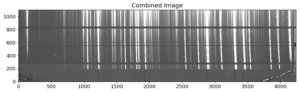
fig = plt.figure(figsize=(12, 6))
ax = fig.add_subplot(111)
vmin, vmax = interval.get_limits(carc.data)
im = ax.imshow(carc.data.T, cmap="gray", origin="lower", vmin=vmin, vmax=vmax)
ax.set_title("Combined Image")

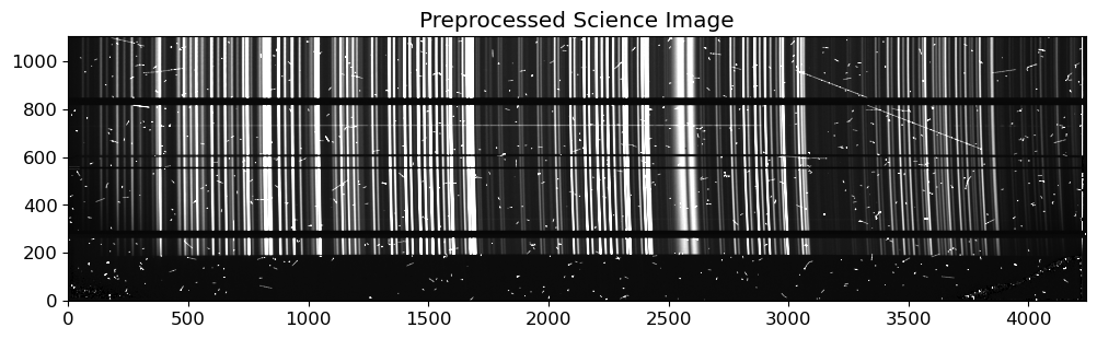
fig = plt.figure(figsize=(12, 6))
ax = fig.add_subplot(111)
sci = fits.getdata(OUTDIR / f"p{sci_list[0].stem}")
vmin, vmax = interval.get_limits(sci)
im = ax.imshow(sci.T, cmap="gray", origin="lower", vmin=vmin, vmax=vmax)
ax.set_title("Preprocessed Science Image")

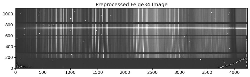
fig = plt.figure(figsize=(12, 6))
ax = fig.add_subplot(111)
std34 = fits.getdata(OUTDIR / f"p{std_list_f34[0].stem}")
vmin, vmax = interval.get_limits(std34)
im = ax.imshow(std34.T, cmap="gray", origin="lower", vmin=vmin, vmax=vmax)
ax.set_title("Preprocessed Feige34 Image")
fig.show()

Wavelength Calibration

Wavelength calibration is the process of converting the pixel coordinates of the spectrum into the corresponding wavelengths. This is typically done by using the arc lamp images, which contain known spectral lines at known wavelengths. The arc lamp images are taken with the same setup as the science images, and the spectral lines in the arc lamp images are used to calibrate the wavelength scale of the science images. On the other hand, in some cases, the sky lines can be used for the wavelength calibration, especially when the arc lamp lines are not available or not reliable. We call these images that contain information for the wavelength calibration “comparison images”.

The wavelength calibration is done by fitting a polynomial to the pixel-wavelength relation, using the 1D spectrum extracted from the comparison images, at initial spatial strip. This process is called “identify” in IRAF, since it is done by identifying the spectral lines in the comparison images and fitting a polynomial to the pixel-wavelength relation.

After the “identify” process, the process called “reidentify” should be performed to construct 2D pixel-wavelength relation. This is done by fitting a polynomial to the pixel-wavelength relation, using the 1D spectrum extracted from the comparison images, at other spatial strips. This process is called “reidentify” in IRAF, since it is done by reidentifying the spectral lines at different positions and fitting a polynomial to the pixel-wavelength relations again.

Region of Interest (RoI)

Region of Interest (RoI) is the region where all the required data for the extraction of science spectrum is located. When we see the above image, a lot portion of the image is not useful for the extraction of the spectrum. Therefore, we need to define the RoI to reduce the computational cost. Let’s define the RoI for all extraction processes, by inspecting the 2D spectrum of the science frames.

# Trim the images
TRIM = [0, 4220, 670, 810]  # y_lower, y_upper, x_lower, x_upper
fname = OUTDIR / f"p{sci_list[0].stem}"
stdhdu = fits.open(fname)
stdhdr = stdhdu[0].header
stdtrim = stdhdu[0].data[TRIM[0] : TRIM[1], TRIM[2] : TRIM[3]]
exptime = stdhdr["EXPTIME"]
rdnoise = stdhdr["RDNOISE"]
pressure = stdhdr["DOM-PRS"]
temperature = stdhdr["DOM-TMP"]
humidity = stdhdr["DOM-HUM"]

fig = plt.figure(figsize=(12, 2))
ax = fig.add_subplot(111)
vmin, vmax = interval.get_limits(stdtrim)
im = ax.imshow(stdtrim.T, cmap="gray", origin="lower", vmin=vmin, vmax=vmax)
ax.set_title("Preprocessed Science Image (Trimmed)")
fig.show()

The TRIM parameter is used to trim the images to the RoI. The elements of the TRIM parameter is determined by examining the 2D science frame, to make the source centered in the image. From now on, we will use the trimmed images for the data reduction process, with the same RoI for all the images.

Identify

Now we can proceed to the wavelength calibration process with following steps:

1. Extract the 1D spectrum of the comparison image: We will extract the 1D spectrum of the comparison image, simply taking a strip from a row (or summation of a few rows) of the comparison image. We will extract the 1D spectrum at the initial spatial strip, and use it to identify the spectral lines.

2. Identify the spectral lines: We will find the line peaks in the 1D spectrum and matching them with the known wavelengths of the spectral lines.

3. Fit a polynomial to the pixel-wavelength relation: We will fit a polynomial to the pixel-wavelength relation, using the pixel coordinates of the line peaks and the known wavelengths of the spectral lines. The degree of the polynomial should be determined by the complexity of the solution.

In this notebook, we will use the arc framesfor the comparison images. However, The FOCAS reduction help page recommends using the sky lines for the wavelength calibration for the VPH900 grism. The sky lines are the emission lines from the Earth’s atmosphere, and they can be used for the wavelength calibration. Especially, our arc lamp images were taken at a few hours earlier than the science frames, and different pointing directions might introduce some deviations for wavelength solutions. Therefore, it is recommended to use the sky lines for the wavelength calibration in this case. In practice, one can use both the sky lines and the arc lamp lines for the wavelength calibration, and compare the results. In this notebook, we will use the arc lamp lines for the wavelength calibration, but you can try using the sky lines for the wavelength calibration as an exercise.

How should we identify the arc lines and assign the wavelengths to them? This task needs manual identification and allocation for the best results. However, it might be very time-consuming, especially when the number of lines is large. There were lots of effort to automate this process, and we can use various softwares such as the autoidentify task in IRAF. In this notebook, we will use the RASCAL package for Python, which is a Python package for automatic spectral line identification and wavelength calibration adopted for the ASPIRED pipeline. For more information on how the RASCAL package works, please refer to the RASCAL documentation.

Before we proceed, install the RASCAL package by running the following command:

pip install rascal

Let’s start from the step 1, extracting the 1D spectrum of the comparison image. Before the extraction, the cosmic ray removal will mitigate some confusion in the identification process.

# Trim the images
fname = OUTDIR / f"cArc.fits"
# fname = OUTDIR / f"p{arc_list[0].stem}"
stdhdu = fits.open(fname)
stdhdr = stdhdu[0].header
stdtrim = stdhdu[0].data[TRIM[0] : TRIM[1], TRIM[2] : TRIM[3]]
exptime = stdhdr["EXPTIME"]
rdnoise = stdhdr["RDNOISE"]
# In case you have vacuum references, you need the followings for vacuum-air conversion
# But we don't have vacuum references in this data, so we don't need them.
pressure = stdhdr["DOM-PRS"]
temperature = stdhdr["DOM-TMP"]
humidity = stdhdr["DOM-HUM"]

fig = plt.figure(figsize=(12, 2))
ax = fig.add_subplot(111)
vmin, vmax = interval.get_limits(stdtrim)
im = ax.imshow(stdtrim.T, cmap="gray", origin="lower", vmin=vmin, vmax=vmax)
ax.set_title("Preprocessed Arc Image (Trimmed)")
fig.show()

# Cosmic ray removal
stdccd = CCDData(data=stdtrim, header=stdhdr, unit="adu")
gcorr = gain_correct(stdccd, gain=stdhdr["GAIN"] * u.electron / u.adu)
crrej = cosmicray_lacosmic(
    gcorr, sigclip=7, readnoise=stdhdr["RDNOISE"] * u.electron, verbose=True
)

Starting 4 L.A.Cosmic iterations
Iteration 1:
12682 cosmic pixels this iteration
Iteration 2:
11006 cosmic pixels this iteration
Iteration 3:
9926 cosmic pixels this iteration
Iteration 4:
9492 cosmic pixels this iteration

fig = plt.figure(figsize=(12, 6))
ax = fig.add_subplot(111)
vmin, vmax = interval.get_limits(crrej.data)
im = ax.imshow(crrej.data.T, cmap="gray", origin="lower", vmin=vmin, vmax=vmax)
ax.set_title("Cosmic Ray Removed Arc Image")
fig.show()

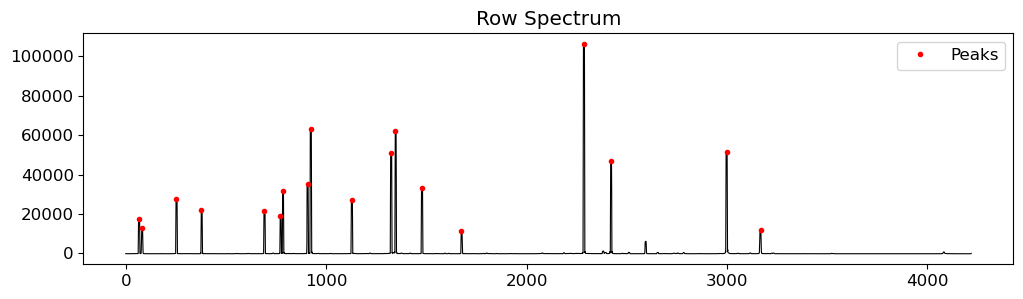
Now we select a few rows from the image to extract the comparison spectrum. I realized that RASCAL does not work well with the inverse order of the spectrum, i.e., the blue side is on the right side. Therefore, we need to flip the spectrum before the identification process.

rowstart = 50  # starting row index for the spectrum
nrows = 3  # number of rows to sum
rowend = rowstart + nrows  # ending row index for the spectrum
rowmid = (rowstart + rowend) / 2  # middle row position for the spectrum
# summing the rows and inverting the spectrum
compspec = crrej.data[:, rowstart:rowend].sum(axis=1)[::-1]

# identify the peaks in the spectrum
peaks = peak_local_max(compspec, min_distance=10, threshold_rel=0.1)

fig = plt.figure(figsize=(12, 3))
ax = fig.add_subplot(111)
ax.plot(compspec, lw=0.8, c="k")
ax.plot(peaks, compspec[peaks], "r.", label="Peaks")
ax.set_title("Row Spectrum")
ax.legend()
fig.show()

We can get the reference wavelength of the arc lines from thar.v900.dat file in the FOCASRED IRAF package (see here).

arclines = Table.read(
    WD / "thar.v900.dat",
    format="ascii.csv",
    names=["wavelength"],
    data_start=1,
)["wavelength"].value

elements = ["ThAr"] * len(arclines)

arclines

array([9784.501 , 9657.7863, 9399.0891, 9354.2198, 9224.4992, 9122.9674,
       8667.9442, 8521.4422, 8424.6475, 8408.2096, 8264.5225, 8115.311 ,
       8103.6931, 8014.7857, 8006.1567, 7948.1764, 7635.106 , 7514.6518,
       7503.8691, 7383.9805, 7272.9359, 7067.2181, 6965.4307, 6911.2264])

# redefine the peaks using the Gaussian fit
peaks_refined = util.refine_peaks(compspec, peaks[:, 0], window_width=5)

# create the RASCAL calibrator object
cal = Calibrator(peaks_refined, compspec)
# set the properties of the calibrator
cal.set_calibrator_properties(
    num_pix=len(compspec), plotting_library="matplotlib", log_level="info"
)
# set the wavelength calibration properties
cal.set_hough_properties(
    num_slopes=5000,
    range_tolerance=500.0,
    xbins=200,
    ybins=200,
    min_wavelength=7500.0,
    max_wavelength=10500.0,
    linearity_tolerance=50.0,
)
# set the model properties
cal.set_ransac_properties(sample_size=5, top_n_candidate=5)

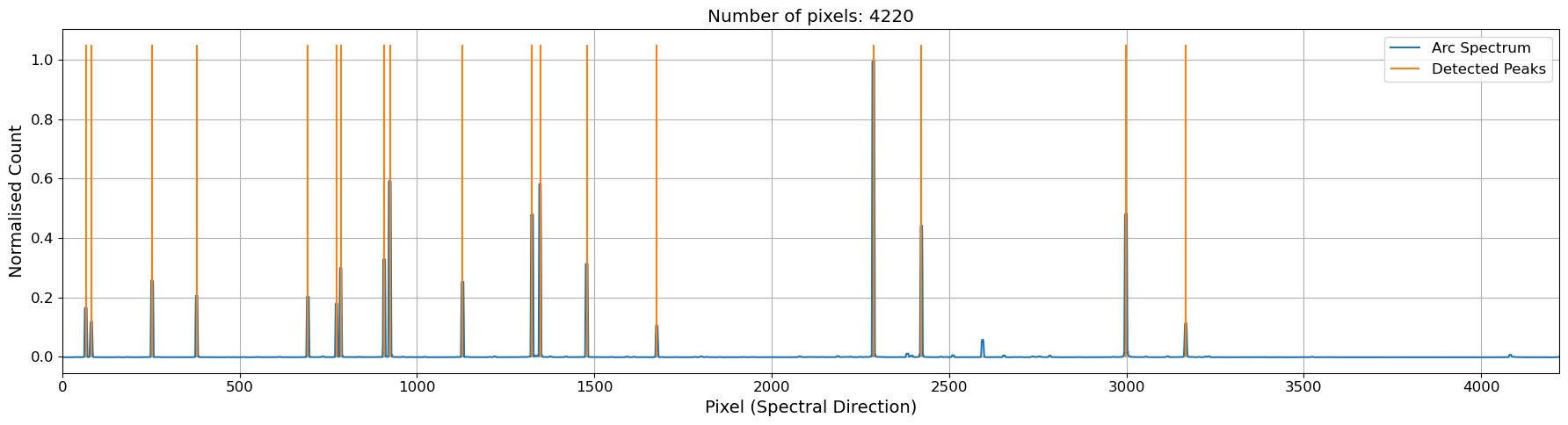
[Wed, 29 May 2024 08:40:21] INFO [calibrator.py:930] num_pix is set to 4220.
[Wed, 29 May 2024 08:40:21] INFO [calibrator.py:942] pixel_list is set to None.
[Wed, 29 May 2024 08:40:21] INFO [calibrator.py:971] Plotting with matplotlib.

cal.plot_arc()
plt.show()

# create an atlas object with the sky lines provided
atlas = Atlas(
    min_atlas_wavelength=8000.0,
    max_atlas_wavelength=10500.0,
    min_intensity=0.0,
)
atlas.add_user_atlas(
    elements=elements,
    wavelengths=arclines,
    vacuum=False,
    pressure=pressure,
    temperature=temperature,
    relative_humidity=humidity,
)

# set the atlas to the calibrator
cal.set_atlas(atlas)

# calibrate the spectrum
cal.do_hough_transform()

# perform chebyshev fit on samples drawn from RANSAC
fit_result = cal.fit(max_tries=100, fit_deg=3)
(
    fit_coeff,
    matched_peaks,
    matched_atlas,
    rms,
    residual,
    peak_utilisation,
    atlas_utilisation,
) = fit_result

rms_reference = rms

[Wed, 29 May 2024 08:40:23] INFO [calibrator.py:750] Found: 17

xidx = np.arange(len(compspec))
wavelength = cal.polyval(xidx, fit_coeff)

fig, axes = plt.subplots(
    3, 1, figsize=(12, 7), gridspec_kw={"height_ratios": [2, 1, 2]}, sharex=True
)
ax1, ax2, ax3 = axes

ax1.plot(wavelength, compspec, lw=0.8, c="k", zorder=3)
labelp, labela = True, True
for peak in peaks_refined:
    if labelp:
        ax1.axvline(
            cal.polyval(peak, fit_coeff), c="tab:red", lw=1, label="Identified Peaks"
        )
        labelp = False
    else:
        ax1.axvline(cal.polyval(peak, fit_coeff), c="tab:red", lw=1)
for atla in arclines:
    if labela:
        ax1.axvline(atla, c="tab:blue", lw=1, label="References", ls="--")
        labela = False
    else:
        ax1.axvline(atla, c="tab:blue", lw=1, ls="--")
ax1.set_ylabel("Counts")
ax1.legend()

wave_matched = cal.polyval(matched_peaks, fit_coeff)
ax2.plot(wave_matched, residual, ls="none", c="k", marker="+")
ax2.axhline(0, c="k", lw=0.5, ls="--")
ax2.text(
    0.99, 0.05, f"RMS: {rms:.2f}", transform=ax2.transAxes, ha="right", va="bottom"
)
ax2.set_ylabel("Residuals [$\AA$]")
ax3.plot(wavelength, xidx, c="tab:green", lw=0.8, label="Solution")
ax3.plot(matched_atlas, matched_peaks, "r+", label="Matched Peaks")
ax3.set_xlabel("Wavelength [$\AA$]")
ax3.set_ylabel("Pixel")
ax3.legend()

fig.subplots_adjust(hspace=0)

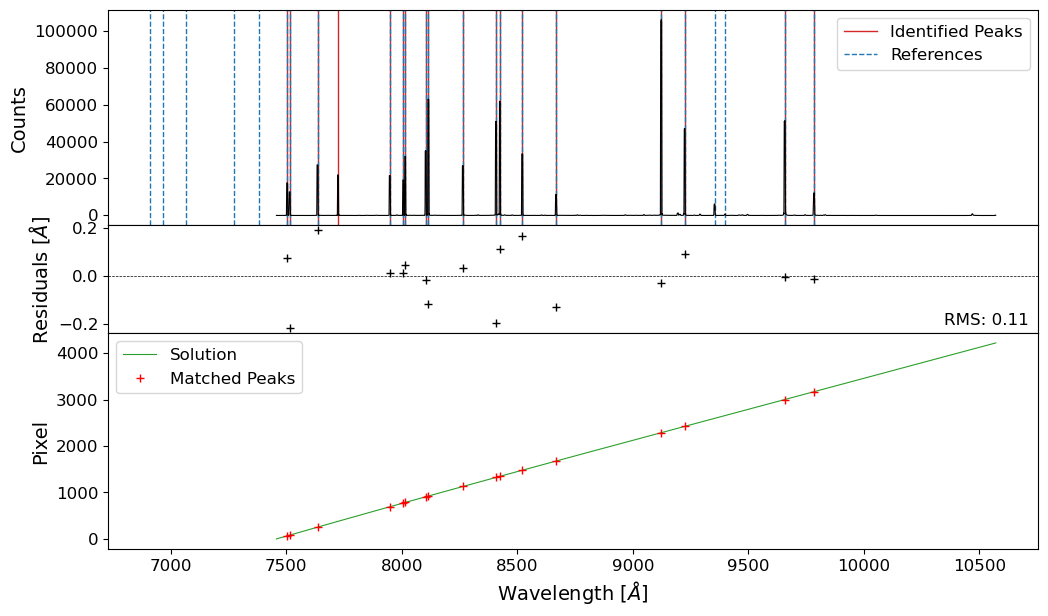
We now have a wavelength solution for the strip of the comparison image, with RMS of 0.17 Angstroms. We can now proceed to the next step, reidentifying to get the 2D pixel-wavelength relation.

Reidentify

The reidentification process is similar to the identification process, but we will use the 1D spectrum extracted from the comparison image at different spatial strips. We will fit a polynomial to the pixel-wavelength relation, using the pixel coordinates of the line peaks and the known wavelengths of the spectral lines. The degree of the polynomial should be determined by the complexity of the solution.

nrows = 3  # number of rows to sum
nintv = 5  # number of intervals between the starting rows
rowstart_array = np.arange(0, crrej.data.shape[1] - nrows, nintv)
rowmid_array = (rowstart_array + rowstart_array + nrows) / 2

list_fit_coeff = []
rms_list = []
list_matched_position = []
for i in range(len(rowstart_array)):
    rowstart = rowstart_array[i]  # starting row index for the spectrum
    rowend = rowstart + nrows  # ending row index for the spectrum
    # summing the rows and inverting the spectrum
    compspec = crrej.data[:, rowstart:rowend].sum(axis=1)[::-1]

    # identify the peaks in the spectrum
    peaks = peak_local_max(compspec, min_distance=10, threshold_rel=0.1)

    # redefine the peaks using the Gaussian fit
    peaks_refined = util.refine_peaks(compspec, peaks[:, 0], window_width=5)

    # create the RASCAL calibrator object
    cal = Calibrator(peaks_refined, compspec)
    # set the properties of the calibrator
    cal.set_calibrator_properties(
        num_pix=len(compspec), plotting_library="matplotlib", log_level="info"
    )
    # set the wavelength calibration properties
    cal.set_hough_properties(
        num_slopes=5000,
        range_tolerance=500.0,
        xbins=200,
        ybins=200,
        min_wavelength=7500.0,
        max_wavelength=10500.0,
        linearity_tolerance=50.0,
    )
    # set the model properties
    cal.set_ransac_properties(sample_size=5, top_n_candidate=5)

    atlas = Atlas(
        min_atlas_wavelength=8000.0,
        max_atlas_wavelength=10500.0,
        min_intensity=0.0,
    )
    atlas.add_user_atlas(
        elements=elements,
        wavelengths=arclines,
        vacuum=False,
        pressure=pressure,
        temperature=temperature,
        relative_humidity=humidity,
    )

    # set the atlas to the calibrator
    cal.set_atlas(atlas)

    # calibrate the spectrum
    cal.do_hough_transform()

    # perform chebyshev fit on samples drawn from RANSAC
    fit_result = cal.fit(max_tries=100, fit_deg=3)
    (
        fit_coeff,
        matched_peaks,
        matched_atlas,
        rms,
        residual,
        peak_utilisation,
        atlas_utilisation,
    ) = fit_result

    save = (rms < 2 * rms_reference) | (len(matched_peaks) > 10)

    if save:
        # append the fit coefficients and rms to the lists
        midrow = np.full_like(matched_peaks, rowmid_array[i])
        list_fit_coeff.append(fit_coeff)
        list_matched_position.append(np.vstack([midrow, matched_peaks, matched_atlas]))
        rms_list.append(rms)

Show code cell output Hide code cell output

[Wed, 29 May 2024 08:40:23] INFO [calibrator.py:930] num_pix is set to 4220.
[Wed, 29 May 2024 08:40:23] INFO [calibrator.py:942] pixel_list is set to None.
[Wed, 29 May 2024 08:40:23] INFO [calibrator.py:971] Plotting with matplotlib.

[Wed, 29 May 2024 08:40:24] INFO [calibrator.py:750] Found: 14
[Wed, 29 May 2024 08:40:24] INFO [calibrator.py:930] num_pix is set to 4220.
[Wed, 29 May 2024 08:40:24] INFO [calibrator.py:942] pixel_list is set to None.
[Wed, 29 May 2024 08:40:24] INFO [calibrator.py:971] Plotting with matplotlib.

[Wed, 29 May 2024 08:40:25] INFO [calibrator.py:750] Found: 16
[Wed, 29 May 2024 08:40:25] INFO [calibrator.py:930] num_pix is set to 4220.
[Wed, 29 May 2024 08:40:25] INFO [calibrator.py:942] pixel_list is set to None.
[Wed, 29 May 2024 08:40:25] INFO [calibrator.py:971] Plotting with matplotlib.

[Wed, 29 May 2024 08:40:26] INFO [calibrator.py:750] Found: 14
[Wed, 29 May 2024 08:40:26] INFO [calibrator.py:930] num_pix is set to 4220.
[Wed, 29 May 2024 08:40:26] INFO [calibrator.py:942] pixel_list is set to None.
[Wed, 29 May 2024 08:40:26] INFO [calibrator.py:971] Plotting with matplotlib.

[Wed, 29 May 2024 08:40:27] INFO [calibrator.py:750] Found: 16
[Wed, 29 May 2024 08:40:27] INFO [calibrator.py:930] num_pix is set to 4220.
[Wed, 29 May 2024 08:40:27] INFO [calibrator.py:942] pixel_list is set to None.
[Wed, 29 May 2024 08:40:27] INFO [calibrator.py:971] Plotting with matplotlib.

[Wed, 29 May 2024 08:40:28] INFO [calibrator.py:750] Found: 15
[Wed, 29 May 2024 08:40:28] INFO [calibrator.py:930] num_pix is set to 4220.
[Wed, 29 May 2024 08:40:28] INFO [calibrator.py:942] pixel_list is set to None.
[Wed, 29 May 2024 08:40:28] INFO [calibrator.py:971] Plotting with matplotlib.

[Wed, 29 May 2024 08:40:29] INFO [calibrator.py:750] Found: 16
[Wed, 29 May 2024 08:40:29] INFO [calibrator.py:930] num_pix is set to 4220.
[Wed, 29 May 2024 08:40:29] INFO [calibrator.py:942] pixel_list is set to None.
[Wed, 29 May 2024 08:40:29] INFO [calibrator.py:971] Plotting with matplotlib.

[Wed, 29 May 2024 08:40:30] INFO [calibrator.py:750] Found: 15
[Wed, 29 May 2024 08:40:30] INFO [calibrator.py:930] num_pix is set to 4220.
[Wed, 29 May 2024 08:40:30] INFO [calibrator.py:942] pixel_list is set to None.
[Wed, 29 May 2024 08:40:30] INFO [calibrator.py:971] Plotting with matplotlib.

[Wed, 29 May 2024 08:40:31] INFO [calibrator.py:750] Found: 15
[Wed, 29 May 2024 08:40:31] INFO [calibrator.py:930] num_pix is set to 4220.
[Wed, 29 May 2024 08:40:31] INFO [calibrator.py:942] pixel_list is set to None.
[Wed, 29 May 2024 08:40:31] INFO [calibrator.py:971] Plotting with matplotlib.

[Wed, 29 May 2024 08:40:32] INFO [calibrator.py:750] Found: 15
[Wed, 29 May 2024 08:40:32] INFO [calibrator.py:930] num_pix is set to 4220.
[Wed, 29 May 2024 08:40:32] INFO [calibrator.py:942] pixel_list is set to None.
[Wed, 29 May 2024 08:40:32] INFO [calibrator.py:971] Plotting with matplotlib.

[Wed, 29 May 2024 08:40:32] INFO [calibrator.py:750] Found: 16
[Wed, 29 May 2024 08:40:32] INFO [calibrator.py:930] num_pix is set to 4220.
[Wed, 29 May 2024 08:40:32] INFO [calibrator.py:942] pixel_list is set to None.
[Wed, 29 May 2024 08:40:32] INFO [calibrator.py:971] Plotting with matplotlib.

[Wed, 29 May 2024 08:40:33] INFO [calibrator.py:750] Found: 17
[Wed, 29 May 2024 08:40:33] INFO [calibrator.py:930] num_pix is set to 4220.
[Wed, 29 May 2024 08:40:33] INFO [calibrator.py:942] pixel_list is set to None.
[Wed, 29 May 2024 08:40:33] INFO [calibrator.py:971] Plotting with matplotlib.

[Wed, 29 May 2024 08:40:34] INFO [calibrator.py:750] Found: 15
[Wed, 29 May 2024 08:40:34] INFO [calibrator.py:930] num_pix is set to 4220.
[Wed, 29 May 2024 08:40:34] INFO [calibrator.py:942] pixel_list is set to None.
[Wed, 29 May 2024 08:40:34] INFO [calibrator.py:971] Plotting with matplotlib.

[Wed, 29 May 2024 08:40:35] INFO [calibrator.py:750] Found: 16
[Wed, 29 May 2024 08:40:35] INFO [calibrator.py:930] num_pix is set to 4220.
[Wed, 29 May 2024 08:40:35] INFO [calibrator.py:942] pixel_list is set to None.
[Wed, 29 May 2024 08:40:35] INFO [calibrator.py:971] Plotting with matplotlib.

[Wed, 29 May 2024 08:40:36] INFO [calibrator.py:750] Found: 16
[Wed, 29 May 2024 08:40:36] INFO [calibrator.py:930] num_pix is set to 4220.
[Wed, 29 May 2024 08:40:36] INFO [calibrator.py:942] pixel_list is set to None.
[Wed, 29 May 2024 08:40:36] INFO [calibrator.py:971] Plotting with matplotlib.

[Wed, 29 May 2024 08:40:37] INFO [calibrator.py:750] Found: 16
[Wed, 29 May 2024 08:40:37] INFO [calibrator.py:930] num_pix is set to 4220.
[Wed, 29 May 2024 08:40:37] INFO [calibrator.py:942] pixel_list is set to None.
[Wed, 29 May 2024 08:40:37] INFO [calibrator.py:971] Plotting with matplotlib.

[Wed, 29 May 2024 08:40:38] INFO [calibrator.py:750] Found: 16
[Wed, 29 May 2024 08:40:38] INFO [calibrator.py:930] num_pix is set to 4220.
[Wed, 29 May 2024 08:40:38] INFO [calibrator.py:942] pixel_list is set to None.
[Wed, 29 May 2024 08:40:38] INFO [calibrator.py:971] Plotting with matplotlib.

[Wed, 29 May 2024 08:40:39] INFO [calibrator.py:750] Found: 16
[Wed, 29 May 2024 08:40:39] INFO [calibrator.py:930] num_pix is set to 4220.
[Wed, 29 May 2024 08:40:39] INFO [calibrator.py:942] pixel_list is set to None.
[Wed, 29 May 2024 08:40:39] INFO [calibrator.py:971] Plotting with matplotlib.

[Wed, 29 May 2024 08:40:40] INFO [calibrator.py:750] Found: 16
[Wed, 29 May 2024 08:40:40] INFO [calibrator.py:930] num_pix is set to 4220.
[Wed, 29 May 2024 08:40:40] INFO [calibrator.py:942] pixel_list is set to None.
[Wed, 29 May 2024 08:40:40] INFO [calibrator.py:971] Plotting with matplotlib.

[Wed, 29 May 2024 08:40:41] INFO [calibrator.py:750] Found: 16
[Wed, 29 May 2024 08:40:41] INFO [calibrator.py:930] num_pix is set to 4220.
[Wed, 29 May 2024 08:40:41] INFO [calibrator.py:942] pixel_list is set to None.
[Wed, 29 May 2024 08:40:41] INFO [calibrator.py:971] Plotting with matplotlib.

[Wed, 29 May 2024 08:40:41] INFO [calibrator.py:750] Found: 16
[Wed, 29 May 2024 08:40:41] INFO [calibrator.py:930] num_pix is set to 4220.
[Wed, 29 May 2024 08:40:41] INFO [calibrator.py:942] pixel_list is set to None.
[Wed, 29 May 2024 08:40:41] INFO [calibrator.py:971] Plotting with matplotlib.

[Wed, 29 May 2024 08:40:42] INFO [calibrator.py:750] Found: 15
[Wed, 29 May 2024 08:40:42] INFO [calibrator.py:930] num_pix is set to 4220.
[Wed, 29 May 2024 08:40:42] INFO [calibrator.py:942] pixel_list is set to None.
[Wed, 29 May 2024 08:40:42] INFO [calibrator.py:971] Plotting with matplotlib.

[Wed, 29 May 2024 08:40:43] INFO [calibrator.py:750] Found: 15
[Wed, 29 May 2024 08:40:43] INFO [calibrator.py:930] num_pix is set to 4220.
[Wed, 29 May 2024 08:40:43] INFO [calibrator.py:942] pixel_list is set to None.
[Wed, 29 May 2024 08:40:43] INFO [calibrator.py:971] Plotting with matplotlib.

[Wed, 29 May 2024 08:40:44] INFO [calibrator.py:750] Found: 15
[Wed, 29 May 2024 08:40:44] INFO [calibrator.py:930] num_pix is set to 4220.
[Wed, 29 May 2024 08:40:44] INFO [calibrator.py:942] pixel_list is set to None.
[Wed, 29 May 2024 08:40:44] INFO [calibrator.py:971] Plotting with matplotlib.

[Wed, 29 May 2024 08:40:45] INFO [calibrator.py:750] Found: 6
[Wed, 29 May 2024 08:40:45] INFO [calibrator.py:930] num_pix is set to 4220.
[Wed, 29 May 2024 08:40:45] INFO [calibrator.py:942] pixel_list is set to None.
[Wed, 29 May 2024 08:40:45] INFO [calibrator.py:971] Plotting with matplotlib.

[Wed, 29 May 2024 08:40:46] INFO [calibrator.py:750] Found: 6
[Wed, 29 May 2024 08:40:46] INFO [calibrator.py:930] num_pix is set to 4220.
[Wed, 29 May 2024 08:40:46] INFO [calibrator.py:942] pixel_list is set to None.
[Wed, 29 May 2024 08:40:46] INFO [calibrator.py:971] Plotting with matplotlib.

[Wed, 29 May 2024 08:40:47] INFO [calibrator.py:750] Found: 9
[Wed, 29 May 2024 08:40:47] INFO [calibrator.py:930] num_pix is set to 4220.
[Wed, 29 May 2024 08:40:47] INFO [calibrator.py:942] pixel_list is set to None.
[Wed, 29 May 2024 08:40:47] INFO [calibrator.py:971] Plotting with matplotlib.

[Wed, 29 May 2024 08:40:48] INFO [calibrator.py:750] Found: 15
[Wed, 29 May 2024 08:40:48] INFO [calibrator.py:930] num_pix is set to 4220.
[Wed, 29 May 2024 08:40:48] INFO [calibrator.py:942] pixel_list is set to None.
[Wed, 29 May 2024 08:40:48] INFO [calibrator.py:971] Plotting with matplotlib.

[Wed, 29 May 2024 08:40:49] INFO [calibrator.py:750] Found: 15

matched_positions = np.hstack(list_matched_position)

# fit a 2D Chebyshev polynomial to the matched positions
order_wavelength_reid = 3
order_spatial_reid = 3
coeff_init = Chebyshev2D(x_degree=order_wavelength_reid, y_degree=order_spatial_reid)
fitter = LevMarLSQFitter()
fit2d_reid = fitter(
    coeff_init, matched_positions[0], matched_positions[1], matched_positions[2]
)

coeff_init_inv = Chebyshev2D(
    x_degree=order_spatial_reid, y_degree=order_wavelength_reid
)
fit2d_reid_inv = fitter(
    coeff_init_inv, matched_positions[0], matched_positions[2], matched_positions[1]
)

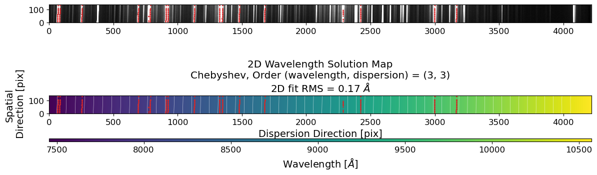
# plot the 2D wavelength solution map and points used for the fit

dd, ss = np.meshgrid(np.arange(crrej.data.shape[0]), np.arange(crrej.data.shape[1]))
rms_reid = np.sqrt(
    np.mean(
        (fit2d_reid(matched_positions[0], matched_positions[1]) - matched_positions[2])
        ** 2
    )
)
wavesol_reid = fit2d_reid(ss, dd)

fig = plt.figure(figsize=(14, 5))
ax = fig.add_subplot(211)
ax.imshow(crrej.data.T[:, ::-1], origin="lower", cmap="gray", vmin=vmin, vmax=vmax)
ax.plot(
    matched_positions[1],
    matched_positions[0],
    c="tab:red",
    label="Matched Peaks",
    marker="+",
    ms=2,
    ls="none",
)
ax = fig.add_subplot(212)
im = ax.imshow(
    wavesol_reid,
    origin="lower",
    cmap="viridis",
)
ax.plot(
    matched_positions[1],
    matched_positions[0],
    c="tab:red",
    label="Matched Peaks",
    marker="+",
    ms=2,
    ls="none",
)
# ax.set_aspect("auto")

ax.contour(
    wavesol_reid,
    colors="w",
    linewidths=0.3,
    levels=np.arange(7500, 10500, 50),
    ls=":",
    zorder=1,
)

divider = make_axes_locatable(ax)
cax = divider.append_axes("bottom", size="15%", pad=0.5)
fig.colorbar(im, cax=cax, orientation="horizontal")

cax.set_xlabel("Wavelength [$\AA$]")
ax.set_xlabel("Dispersion Direction [pix]")
ax.set_ylabel("Spatial\n Direction [pix]")
ax.set_title(
    f"2D Wavelength Solution Map\n"
    + "Chebyshev, Order (wavelength, dispersion) = "
    + f"({order_wavelength_reid}, {order_spatial_reid})\n"
    + f"2D fit RMS = {rms_reid:.2f} $\AA$"
)

Text(0.5, 1.0, '2D Wavelength Solution Map\nChebyshev, Order (wavelength, dispersion) = (3, 3)\n2D fit RMS = 0.17 $\\AA$')

# check the wavelength interval between the pixels
mean_intv = (
    np.mean(np.max(wavesol_reid, axis=1) - np.min(wavesol_reid, axis=1))
    / crrej.data.shape[0]
)
mean_intv
# make a wavelength grid
wavegrid = np.arange(7500, 10200, mean_intv)

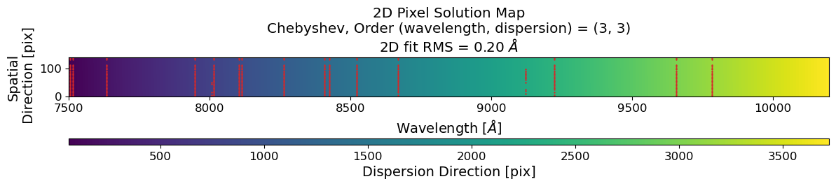
# plot the 2D dispersion solution map and points used for the fit

ww, ss = np.meshgrid(wavegrid, np.arange(crrej.data.shape[1]))
rms_reid_inv = np.sqrt(
    np.mean(
        (
            fit2d_reid_inv(matched_positions[0], matched_positions[2])
            - matched_positions[1]
        )
        ** 2
    )
)
disp_reid = fit2d_reid_inv(ss, ww)

fig = plt.figure(figsize=(14, 3))
ax = fig.add_subplot(111)
im = ax.imshow(
    disp_reid,
    origin="lower",
    cmap="viridis",
    extent=[wavegrid[0], wavegrid[-1], 0, disp_reid.shape[0]],
)
ax.plot(
    matched_positions[2],
    matched_positions[0],
    c="tab:red",
    label="Matched Peaks",
    marker="+",
    ms=2,
    ls="none",
)

divider = make_axes_locatable(ax)
cax = divider.append_axes("bottom", size="15%", pad=0.6)
fig.colorbar(im, cax=cax, orientation="horizontal")

cax.set_xlabel("Dispersion Direction [pix]")
ax.set_xlabel("Wavelength [$\AA$]")
ax.set_ylabel("Spatial\n Direction [pix]")
ax.set_title(
    f"2D Pixel Solution Map\n"
    + "Chebyshev, Order (wavelength, dispersion) = "
    + f"({order_wavelength_reid}, {order_spatial_reid})\n"
    + f"2D fit RMS = {rms_reid_inv*mean_intv:.2f} $\AA$"
)
plt.show()

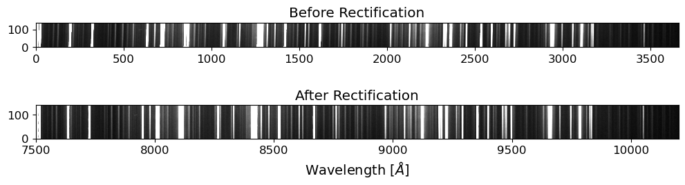
Rectify the 2D Spectrum

After the reidentification process, we will rectify the 2D spectrum by applying the wavelength solution to the 2D spectrum. This will convert the pixel coordinates of the spectrum into the corresponding wavelengths. The rectified 2D spectrum will be used for the extraction of the 1D spectrum.

For the rectification process, we will use the map_coordinates function from the scipy package. The map_coordinates function interpolates the pixel values of the input image at the given coordinates.

xycoords = np.vstack([disp_reid.ravel(), ss.ravel()])
rectified = map_coordinates(
    crrej.data[::-1, :], xycoords, mode="constant", cval=0
).reshape(ss.shape)

disp_reid[0]

array([  59.44351046,   60.49814155,   61.55272016, ..., 3718.73271463,
       3719.72205358, 3720.7114093 ])

fig, axes = plt.subplots(2, 1, figsize=(12, 3))
ax = axes[0]
ax.imshow(
    crrej.data[::-1, :].T[:, 59:3721], origin="lower", cmap="gray", vmin=vmin, vmax=vmax
)
ax.set_title("Before Rectification")
ax = axes[1]
ax.imshow(
    rectified,
    origin="lower",
    cmap="gray",
    vmin=vmin,
    vmax=vmax,
    extent=[wavegrid[0], wavegrid[-1], 0, rectified.shape[0]],
)
ax.set_title("After Rectification")
ax.set_xlabel("Wavelength [$\AA$]")

Text(0.5, 0, 'Wavelength [$\\AA$]')

Extracting 1D Spectra

The 1D spectra are extracted from the 2D science frames by summing the flux along the spatial direction. The extraction process consists of the following steps:

1. Source Identification: Identify the source in the 2D science frame.

2. Aperture Tracing: Trace the spatial position of the source along the dispersion direction.

3. Aperture Summation: Sum the flux along the trace to extract the 1D spectrum.

Let’s extract the 1D spectra of the standard star first, because it is brighter and easier to extract.

1. Source Identification

Let’s trim the images to the region of interest. Then, after the cosmic ray removal, we will identify the source in the 2D science frame. We will use the peak_local_max function from skimage.feature module to identify the source in a slice of the 2D science frame. The peak_local_max function finds the local maxima, which can be used to identify the source in the 2D science frame.

# Trim the images
TRIM = [0, 4220, 670, 810]  # y_lower, y_upper, x_lower, x_upper
fname = OUTDIR / f"p{std_list_f34[0].stem}"
stdhdu = fits.open(fname)
stdhdr = stdhdu[0].header
stdtrim = stdhdu[0].data[TRIM[0] : TRIM[1], TRIM[2] : TRIM[3]]
exptime = stdhdr["EXPTIME"]
rdnoise = stdhdr["RDNOISE"]

fig = plt.figure(figsize=(12, 2))
ax = fig.add_subplot(111)
vmin, vmax = interval.get_limits(stdtrim)
im = ax.imshow(stdtrim.T, cmap="gray", origin="lower", vmin=vmin, vmax=vmax)
ax.set_title("Preprocessed Feige34 Image (Trimmed)")
fig.show()

Cosmic ray removal often takes a long time. Hence, we will apply cosmic ray removal on the trimmed images to save unnecessary computation. To get reliable removal of cosmic rays, we need to mask bad pixels, but here we will skip this step for simplicity. For more information on cosmic ray removal, please refer to the CCD Data Reduction Guide.

# Cosmic ray removal
stdccd = CCDData(data=stdtrim, header=stdhdr, unit="adu")
gcorr = gain_correct(stdccd, gain=stdhdr["GAIN"] * u.electron / u.adu)
crrej = cosmicray_lacosmic(
    gcorr, sigclip=7, readnoise=stdhdr["RDNOISE"] * u.electron, verbose=True
)

Starting 4 L.A.Cosmic iterations
Iteration 1:
325 cosmic pixels this iteration
Iteration 2:
34 cosmic pixels this iteration
Iteration 3:
21 cosmic pixels this iteration
Iteration 4:
19 cosmic pixels this iteration

Show code cell source Hide code cell source

fig = plt.figure(figsize=(12, 6))
ax = fig.add_subplot(111)
vmin, vmax = interval.get_limits(crrej.data)
im = ax.imshow(crrej.data.T, cmap="gray", origin="lower", vmin=vmin, vmax=vmax)
ax.set_title("Cosmic Ray Removed Feige34 Image")
fig.show()

# Flip and Rectify the Feige34 image
rectified = map_coordinates(
    crrej.data[::-1, :], xycoords, mode="constant", cval=0
).reshape(ss.shape)

fig = plt.figure(figsize=(12, 3))
ax = fig.add_subplot(111)
ax.imshow(rectified, origin="lower", cmap="gray", vmin=vmin, vmax=vmax)
ax.set_title("Flipped and Rectified Feige34 Image")
fig.show()

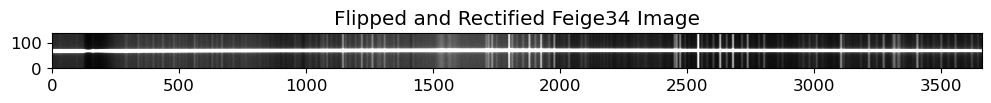
Looks good. Now we will identify the source position.

# Slice the image in the spatial direction
lcut = 1000  # left cut (dispersion direction)
rcut = 1050  # right cut (dispersion direction)

apall_probe = np.sum(rectified[:, lcut:rcut], axis=1)
x_probe = np.arange(apall_probe.size)
peak_pix = peak_local_max(
    apall_probe, num_peaks=1, min_distance=50, threshold_abs=np.median(apall_probe)
)[0][0]
print("Peak pixel:", peak_pix)

Peak pixel: 68

Show code cell source Hide code cell source

fig = plt.figure(figsize=(6, 4))
ax = fig.add_subplot(111)
ax.step(x_probe, apall_probe, where="mid")
ax.plot(
    (peak_pix, peak_pix),
    (
        apall_probe[peak_pix] + 0.01 * apall_probe[peak_pix],
        apall_probe[peak_pix] + 0.05 * apall_probe[peak_pix],
    ),
    c="tab:red",
)
ax.annotate(
    peak_pix,
    (peak_pix, apall_probe[peak_pix] + 0.05 * apall_probe[peak_pix]),
    textcoords="offset points",
    xytext=(0, 10),
    ha="left",
    va="top",
    color="k",
    fontsize="small",
    rotation=45,
)
ax.set_title("Aperture Sum")
ax.set_xlabel("Pixel Number (Spatial Direction)")
ax.set_ylabel("Counts [e-]")
fig.show()

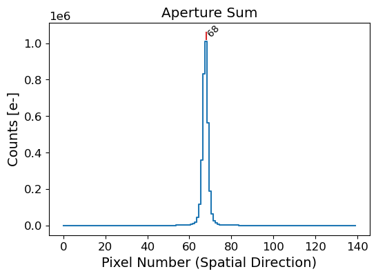
Here we crop the image in the dispersion direction, from lcut to rcut. We sum the counts in the dispersion direction to get the 1D spatial profile of the source. We then use the peak_local_max function to identify the source position in the spatial profile. The peak_local_max function finds the local maxima in the 1D profile, which can be used to identify the source position. Then we can also estimate the full width at half maximum (FWHM) of the source, using the peak_widths function from the scipy.signal module.

From the above figure, we were able to get the pixel position of the peak of the source. However, the peak position is not always the center of the source, since it is an integer value. Therefore, we need some centering algorithm to get the center of the source to properly trace the spatial position of the source along the dispersion axis.

Here we use the centroid_com function from the photutils package to get the center of the source. The centroid_com function calculates the center of mass of the source, which is a good approximation of the center of the source. This function originally calculate the centroid of the source in the 2D image, but we will use them to calculate the center of the source in the 1D spatial profile. For more information on centroiding, please refer to the photutils documentation.

Before we estimate the center of the source, we need to estimate the background level. The background level is estimated by fitting a polynomial to the 1D spatial profile of the source. The background level is then subtracted from the 1D spatial profile to get the background-subtracted profile. The background-subtracted profile is then used to estimate the center of the source.

Let’s estimate the background level and subtract it from the 1D spatial profile. Here we use a Chebyshev polynomial of degree 3. The degree of the polynomial can be adjusted depending on the complexity of the background. To model the background, we should set the sky region where the source is not present. The sky region should be chosen carefully to avoid any contamination from the source.

# Select the sky region for the background estimation
sky_limit_peak = 10  # pixel limit from the peak pixel

mask_sky = np.ones_like(apall_probe, dtype=bool)
mask_sky[peak_pix - sky_limit_peak : peak_pix + sky_limit_peak] = False

x_probe_sky = x_probe[mask_sky]
apall_probe_sky = apall_probe[mask_sky]

fig = plt.figure(figsize=(6, 4))
ax = fig.add_subplot(111)
ax.step(x_probe, apall_probe, where="mid")
ax.fill_between(
    x_probe, 0, 1, where=mask_sky, alpha=0.1, transform=ax.get_xaxis_transform()
)
ax.set_xlabel("Pixel Number (Spatial Direction)")
ax.set_ylabel("Counts [e-]")

Text(0, 0.5, 'Counts [e-]')

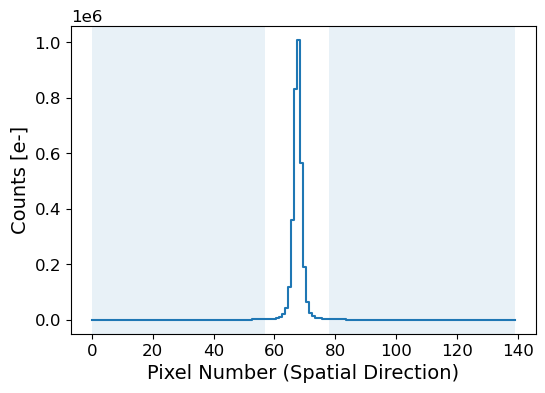
# Fit the sky background with a Chebyshev polynomial
# define function for background fitting
def fit_background(x, apall, fitmask, sigma_sigclip, order_skymodel):
    x_sky = x[fitmask]
    apall_sky = apall[fitmask]
    # sigma clipping
    mask_sigclip = sigma_clip(apall_sky, sigma=sigma_sigclip, masked=True).mask

    # fitting the sky background
    coeffs_sky, fitfull_sky = chebfit(
        x_sky[~mask_sigclip],
        apall_sky[~mask_sigclip],
        deg=order_skymodel,
        full=True,
    )

    # sky background model
    x = np.arange(apall.size)
    skymodel = chebval(x, coeffs_sky)

    # calculating the rms
    residual_skymodel = fitfull_sky[0][0]
    rms_skymodel = np.sqrt(residual_skymodel / len(x_sky[~mask_sigclip]))

    return skymodel, rms_skymodel, mask_sigclip

# setting the parameters
sigma_sigclip = 3
order_skymodel = 3

# fitting the sky background
skymodel, rms_skymodel, mask_sigclip = fit_background(
    x_probe,
    apall_probe,
    mask_sky,
    sigma_sigclip=sigma_sigclip,
    order_skymodel=order_skymodel,
)

# number of pixels
npix_sky = len(x_probe_sky)
npix_skymodel = np.count_nonzero(~mask_sigclip)

Show code cell source Hide code cell source

fig, axes = plt.subplots(2, 1, figsize=(12, 8), gridspec_kw={"height_ratios": [4, 1]})
ax = axes[0]
ax.step(x_probe, apall_probe, where="mid")
ax.fill_between(
    x_probe, 0, 1, where=mask_sky, alpha=0.1, transform=ax.get_xaxis_transform()
)

ax.plot(
    x_probe,
    skymodel,
    c="tab:red",
    lw=1,
    label=f"Chebyshev Sky Model ({npix_skymodel:d}/{npix_sky:d})",
)
ax.plot(
    x_probe_sky[mask_sigclip],
    apall_probe_sky[mask_sigclip],
    "x",
    c="tab:orange",
    label=f"Sigma-clipped ({sigma_sigclip:.1f}-sigma)",
)

resax = axes[1]
resax.plot([0, x_probe[-1]], [0, 0], c="k", ls="--", lw=0.8)
resax.step(
    x_probe, apall_probe - skymodel, where="mid", label=f"RMS={rms_skymodel:.2f}"
)
resax.fill_between(
    x_probe,
    0,
    1,
    where=mask_sky,
    color="tab:blue",
    alpha=0.1,
    transform=resax.get_xaxis_transform(),
)
resax.plot(
    x_probe_sky[mask_sigclip],
    apall_probe_sky[mask_sigclip] - skymodel[mask_sky][mask_sigclip],
    "x",
    c="tab:orange",
)
resax.set_xlabel("Pixel Number (Spatial Direction)")
resax.set_ylabel("Residuals [e-]")
# ylim_ax = ax.get_ylim()
ylim_resax = rms_skymodel * np.array([-1, 1]) * 10
resax.set_ylim(ylim_resax)
resax.tick_params(axis="x", direction="in", top="on")
resax.legend()

title_str = f"Skyfit: Chebyshev order {order_skymodel:d} ({sigma_sigclip:.1f}-sigma)"
ax.tick_params(axis="x", direction="in", labelbottom=False)
ax.set_xlabel("Pixel Number (Spatial Direction)")
ax.set_ylabel("Counts [e-]")
ax.set_title(title_str)
ax.legend()

for aa in axes:
    aa.set_xlim(0, x_probe[-1])

fig.subplots_adjust(hspace=0)

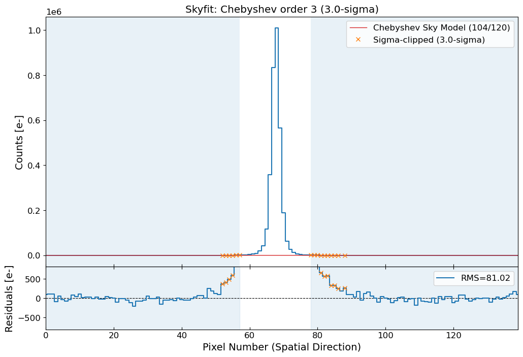
From the sigma clipping, we can see some rejected points near the source. This indicates that the sky region we set is not sufficiently far from the source. We should set the sky region further away from the source to avoid any contamination from the source. Sigma clipping will also reject any cosmic rays or bad pixels in the sky region, which will affect the background estimation.

from photutils.centroids import centroid_com

apall_probe_skysub = apall_probe - skymodel

center_probe_com = centroid_com(apall_probe_skysub)[0]
print("Center without sky subtraction:", centroid_com(apall_probe)[0])
print("Center after sky subtraction:", center_probe_com)

pwresult = peak_widths(apall_probe_skysub, [peak_pix], rel_height=0.5)
fwhm_probe = pwresult[0][0]
left_ips, right_ips = pwresult[2][0], pwresult[3][0]
fwhm_hight = pwresult[1][0]
print("FWHM:", fwhm_probe)
print("Left and right interpolated positions:", left_ips, right_ips)

Center without sky subtraction: 67.73007980094286
Center after sky subtraction: 67.73009569607028
FWHM: 2.8507875970919656
Left and right interpolated positions: 66.30838212291202 69.15916972000399

Show code cell source Hide code cell source

fig = px.line(
    x=np.arange(len(apall_probe_skysub)),
    y=apall_probe,
    title="Sky Subtracted Sum",
    labels={"x": "Pixel Number (Spatial Direction)", "y": "Counts [e-]"},
    line_shape="hvh",
)

fig.add_vline(
    x=peak_pix,
    line_dash="dash",
    line_color="red",
    annotation_text="Peak",
    annotation_position="top right",
    line_width=0.8,
)

fig.add_vline(
    x=center_probe_com,
    line_dash="dash",
    line_color="green",
    annotation_text="Center",
    annotation_position="top left",
    line_width=0.8,
)

fig.add_trace(
    go.Scatter(
        x=[left_ips, right_ips],
        y=[fwhm_hight, fwhm_hight],
        mode="lines+markers",
        line=dict(color="red", width=1.5),
        name=f"FWHM={fwhm_probe:.2f}",
    )
)

fig

Zoom in to see the subtle difference between the peak position and the center position.

2. Aperture Tracing

We have identified the source position in the spatial direction by collapsing a slice of the 2D science frame along the dispersion direction. Next, we will trace the spatial position of the source along the dispersion direction. This involves changing the location of the slices in the dispersion direction and identifying the source position in each slice.

# Define the function for determining the center of the source for given slice range
def get_skymask(apall, sky_limit_peak, center=None):
    if center is None:
        peak_pix = peak_local_max(
            apall,
            num_peaks=1,
            min_distance=10,
            threshold_abs=np.mean(apall),
        )[0][0]
    else:
        peak_pix = round(center)

    mask_sky = np.ones_like(apall, dtype=bool)
    mask_sky[peak_pix - sky_limit_peak : peak_pix + sky_limit_peak] = False

    return mask_sky, peak_pix


def find_center(data, lcut, rcut, sky_limit_peak, sigma_sigclip, order_skymodel):
    apall = np.sum(data[:, lcut:rcut], axis=1)
    x = np.arange(apall.size)

    # mask for the sky region and initial peak pixel
    mask_sky, peak_pix = get_skymask(apall, sky_limit_peak)

    # fitting the sky background
    skymodel, rms_skymodel, mask_sigclip = fit_background(
        x,
        apall,
        mask_sky,
        sigma_sigclip=sigma_sigclip,
        order_skymodel=order_skymodel,
    )

    apall_skysub = apall - skymodel

    # center of the source
    center_com = centroid_com(apall_skysub)[0]

    # fwhm of the source
    pwresult = peak_widths(apall_skysub, [round(peak_pix)], rel_height=0.5)
    fwhm = pwresult[0][0]

    return center_com, fwhm


# Find the center of the source for all the slices
slice_width = 50
sky_limit_peak = 20  # increased the distance from the source
midpoints = []
aptrace = []
aptrace_fwhm = []
lcut, rcut = 0, slice_width
while rcut < rectified.shape[1]:
    rcut = lcut + slice_width
    midpoints.append((lcut + rcut) / 2)
    center, fwhm = find_center(
        rectified, lcut, rcut, sky_limit_peak, sigma_sigclip, order_skymodel
    )
    aptrace.append(center)
    aptrace_fwhm.append(fwhm)
    lcut += slice_width
    rcut += slice_width

aptrace = np.array(aptrace)
aptrace_fwhm = np.array(aptrace_fwhm)
aptrace_sigma = aptrace_fwhm * gaussian_fwhm_to_sigma
midpoints = np.array(midpoints)

# Let's fit the aperture trace
order_aptrace = 9
sigma_clip_aptrace = 3

# fitting the trace line
coeffs_aptrace_init = chebfit(midpoints, aptrace, deg=order_aptrace)

# sigma clipping
mask_aptrace = sigma_clip(
    aptrace - chebval(midpoints, coeffs_aptrace_init),
    sigma=sigma_clip_aptrace,
    masked=True,
).mask

# fitting the trace line again
coeffs_aptrace = chebfit(
    midpoints[~mask_aptrace], aptrace[~mask_aptrace], deg=order_aptrace
)
residuals_aptrace = aptrace - chebval(midpoints, coeffs_aptrace)
rejected = ~np.in1d(midpoints, midpoints[~mask_aptrace])
rms_aptrace = np.sqrt(np.mean(residuals_aptrace[~mask_aptrace] ** 2))

# aperture trace model
ximg = np.arange(rectified.shape[1])
aptrace_model = chebval(ximg, coeffs_aptrace)

Show code cell source Hide code cell source

# plot the aperture trace
%matplotlib inline
fig, axes = plt.subplots(2, 1, figsize=(12, 6), gridspec_kw={"height_ratios": [3, 1]})
ax = axes[0]
ax.imshow(rectified, cmap="gray", origin="lower", vmin=vmin, vmax=vmax, aspect="auto")
ax.scatter(midpoints, aptrace, marker="+", c="dodgerblue", s=100, lw=2, label="Data")
ax.scatter(
    midpoints[rejected],
    aptrace[rejected],
    marker="x",
    c="salmon",
    s=100,
    lw=1,
    label="Rejected",
)
ax.plot(ximg, aptrace_model, c="tab:red", lw=1, label="Chebyshev Trace Model")
ax.plot(midpoints, aptrace + 5 * aptrace_sigma, c="r", lw=0.8, ls="--", label="5-sigma")
ax.plot(midpoints, aptrace - 5 * aptrace_sigma, c="r", lw=0.8, ls="--")
ax.plot(
    midpoints, aptrace + 10 * aptrace_sigma, c="r", lw=0.8, ls=":", label="10-sigma"
)
ax.plot(midpoints, aptrace - 10 * aptrace_sigma, c="r", lw=0.8, ls=":")
ax.set_title("Aperture Trace")
ax.set_ylabel("Pixel Number (Spatial Direction)")
ax.set_xticks([])
ax.legend()

resax = axes[1]
resax.plot([0, ximg[-1]], [0, 0], c="k", ls="--", lw=0.8)
resax.scatter(midpoints, residuals_aptrace, marker="+", c="dodgerblue", s=100, lw=2)
resax.scatter(
    midpoints[rejected],
    residuals_aptrace[rejected],
    marker="x",
    c="salmon",
    s=100,
    lw=1,
)
resax.set_xlabel("Pixel Number (Dispersion Direction)")
resax.set_ylabel("Residuals [pix]")
resax.tick_params(axis="x", direction="in", top="on")
resax_ylim = np.max(np.abs(residuals_aptrace)) * np.array([-1, 1])
resax.set_ylim(resax_ylim)
resax.set_xlim(0, ximg[-1])
resax.text(
    0.99,
    0.95,
    f"RMS={rms_aptrace:.2f}",
    transform=resax.transAxes,
    ha="right",
    va="top",
)

fig.subplots_adjust(hspace=0)

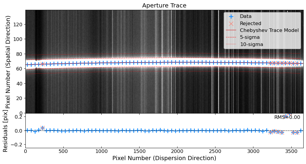
3. Aperture Summation

Now we have traced the spatial position of the source along the dispersion direction. We will sum the flux along the trace to extract the 1D spectrum. The aperture size should be chosen carefully to avoid any contamination from the sky or other sources. The aperture size should be large enough to capture sufficient amount of the flux from the source but small enough to avoid any contamination from the sky or other sources.

See also

The type of aperture used for the extraction can affect the signal-to-noise ratio of the extracted spectrum. One can use a simple aperture, which sums the flux within a fixed aperture size, or an optimal extraction (Horne 1986), which weights the flux based on the spatial profile of the source. The optimal extraction can improve the signal-to-noise ratio of the extracted spectrum, especially when the source is extended or the background is not uniform. In this tutorial, we will use a simple aperture for the extraction, but you can try the optimal extraction for better results.

Let’s make a simple aperture summation to extract the 1D spectrum!

# Define the function for aperture summation
def aperture_sum(
    cut, center, apsum_sigma, ap_sigma, sky_limit_peak, sigma_sigclip, order_skymodel
):
    x = np.arange(len(cut))

    mask_sky, peak_pix = get_skymask(cut, sky_limit_peak, center)
    # aperture size = trace center +/- apsum_sigma * ap_sigma
    appos_lower = int(center - apsum_sigma * ap_sigma)
    appos_upper = int(center + apsum_sigma * ap_sigma)

    # fitting the sky background
    skymodel, rms_skymodel, mask_sigclip = fit_background(
        x,
        cut,
        mask_sky,
        sigma_sigclip=sigma_sigclip,
        order_skymodel=order_skymodel,
    )

    # subtracting the sky background
    cut_skysub = cut - skymodel
    source = cut_skysub[appos_lower:appos_upper]

    # aperture sum
    ap_sum = np.sum(source)

    # calculating the uncertainty
    sig = rdnoise**2 + source + skymodel[appos_lower:appos_upper]
    ap_sig = np.sqrt(np.sum(sig))

    return ap_sum, ap_sig


# Parameters for the aperture summation
apsum_sigma = 10
ap_fwhm = np.median(aptrace_fwhm[~mask_aptrace])  # median FWHM in pixels
ap_sigma = ap_fwhm * gaussian_fwhm_to_sigma  # sigma under the Gaussian assumption

# Extract the spectrum along the dispersion direction
ap_sum = []
ap_sig = []

for i in range(rectified.shape[1]):
    cut_i = rectified[:, i]
    center_i = aptrace_model[i]

    ap_sum_i, ap_sig_i = aperture_sum(
        cut_i,
        center_i,
        apsum_sigma,
        np.median(ap_sigma),
        sky_limit_peak,
        sigma_sigclip,
        order_skymodel,
    )
    ap_sum.append(ap_sum_i)
    ap_sig.append(ap_sig_i)

ap_sum = np.array(ap_sum) / exptime
ap_sig = np.array(ap_sig) / exptime

Show code cell source Hide code cell source

# Plot the extracted spectrum
fig = go.Figure()
fig.add_trace(
    go.Scatter(
        x=wavegrid,
        y=ap_sum,
        error_y=dict(
            type="data",
            array=ap_sig,
            visible=True,
            color="dodgerblue",
            thickness=1,
            width=1,
        ),
        mode="lines+markers",
        marker=dict(color="black", size=3),
        line=dict(color="black", width=0.8),
    )
)
fig.update_layout(
    title="Extracted Spectrum of Feige34",
    xaxis_title="Wavelength [Å]",
    yaxis_title="Counts per Exposure Time[e-/s]",
    showlegend=False,
)
fig

Extracting Spectra of All the Standard Star Frames

I made a python class to extract the 1D spectra from given 2D frames. You can find the class in the apallutils.py script. The class inherits all the frame-specific variables and can be used to extract the 1D spectra from all the frames. You can find the code in our GitHub repository.

from apallutils import InstrumentalSpectrum

std_insspecs = []
for std in std_list_f34:
    fname = OUTDIR / f"p{std.stem}"
    ins = InstrumentalSpectrum(
        fname,
        sky_limit_peak=20,
        sigma_sigclip=3,
        order_skymodel=3,
        order_aptrace=9,
        sigma_clip_aptrace=3,
        slice_width_aptrace=50,
        apsum_sigma=10,
    )
    ins.get_rectified(xycoords, ss.shape, wavegrid)
    ins.set_aptrace()
    ins.set_apsum()
    std_insspecs.append(ins)

Show code cell source Hide code cell source

fig = go.Figure()
f, axes = plt.subplots(3, 1, figsize=(12, 3))
i = 0
for StdInsSpec in std_insspecs:
    ax = axes[i]
    fig.add_trace(
        go.Scatter(
            x=ximg,
            y=StdInsSpec.ap_sum,
            error_y=dict(
                type="data",
                array=StdInsSpec.ap_sig,
                visible=True,
                thickness=1,
                width=1,
            ),
            mode="lines+markers",
            marker=dict(size=3),
            line=dict(width=0.8),
            name=StdInsSpec.fname.stem,
        )
    )
    i += 1
    ax.imshow(
        StdInsSpec.crrej.data.T,
        cmap="gray",
        origin="lower",
        vmin=vmin,
        vmax=vmax,
    )
    ax.set_title(StdInsSpec.fname.stem)
f.suptitle("2D Images of the Standard Star Frames")
fig.update_layout(
    title="Extracted Spectrum of Feige34",
    xaxis_title="Pixel Number (Dispersion Direction)",
    yaxis_title="Counts per Exposure Time[e-/s]",
    showlegend=True,
    legend=dict(yanchor="top", y=0.99, xanchor="left", x=0.01),
)
fig

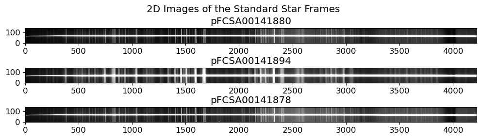
stdtab_f34

Table length=3

filename	date-obs	object	ra	dec	type	exptime	airmass	altitude	disperser	slit-width	slit-pa	slit	filter1	filter2	filter3	ut-str	ut-end
str50	str50	str50	str50	str50	str50	float64	float64	float64	str50	float64	float64	str50	str50	str50	str50	str50	str50
FCSA00141880.fits.gz	2013-06-07	Feige34	10:39:30.972	+43:06:49.26	OBJECT	60.0	1.188	57.2701	SCFCGRHD90	0.5	-240.3	SCFCSLLC08	NONE	SCFCFLSO58	NONE	05:49:08.496	05:50:08.794
FCSA00141894.fits.gz	2013-06-07	Feige34	10:39:30.923	+43:06:49.54	OBJECT	60.0	1.207	55.9261	SCFCGRHD90	0.5	-240.3	SCFCSLLC20	NONE	SCFCFLSO58	NONE	05:58:05.720	05:59:05.978
FCSA00141878.fits.gz	2013-06-07	Feige34	10:39:30.978	+43:06:49.28	OBJECT	60.0	1.185	57.5049	SCFCGRHD90	0.5	-240.3	SCFCSLLC08	NONE	SCFCFLSO58	NONE	05:47:32.380	05:48:32.720

As you can see from the figure above, each extracted spectrum shows different level of continuum. It can be due to various reasons, such as different amount of slit loss due to slight shifts of the source positions with respect to the slit aperture, or the difference in the seeing condition, out-of-focus, etc. To correct this, we can normalize the extracted spectrum by dividing it by the continuum level at some range. Here we will normalize the extracted spectrum by dividing it by the median value of the continuum level at the range of 500-600 pixels.

Note

If we manipulate the continuum level of standard star like this, how should we calibrate the flux of the science frame and trust them? For this reason, we need a process called aperture correction to correct the flux. We will skip this process for simplicity, but you should always consider this process in your own data reduction.

std_norm_factor = np.ones(len(std_insspecs))
refwindow = [500, 600]
for i, StdInsSpec in enumerate(std_insspecs):
    std_norm_factor[i] = np.sum(StdInsSpec.ap_sum[refwindow[0] : refwindow[1]])

# normalize to the maximum value
std_norm_factor = std_norm_factor / np.max(std_norm_factor)

for i, StdInsSpec in enumerate(std_insspecs):
    StdInsSpec.ap_sum /= std_norm_factor[i]
    StdInsSpec.ap_sig /= std_norm_factor[i]

fig = go.Figure()
for i in range(len(std_insspecs)):
    fig.add_trace(
        go.Scatter(
            x=wavegrid,
            y=std_insspecs[i].ap_sum,
            error_y=dict(
                type="data",
                array=std_insspecs[i].ap_sig,
                visible=True,
                thickness=1,
                width=1,
            ),
            mode="lines+markers",
            marker=dict(size=3),
            line=dict(width=0.8),
            name=std_insspecs[i].fname.stem,
        )
    )
fig.update_layout(
    title=" Extracted Spectrum of Feige34 Normalized to the Maximum Value",
    xaxis_title="Wavelength [Å]",
    yaxis_title="Counts per Exposure Time[e-/s]",
    showlegend=True,
    legend=dict(yanchor="top", y=0.99, xanchor="left", x=0.01),
)
fig

If you closely examine the extracted spectra, you will see that there are some shifts in the atmospheric absorption lines. However, the continuum of the standard star shows a good match, indicating that the wavelength solution might be consistent for all the extracted spectra. Still, the shifted frame is taken at different airmass and a different pointing direction. Thus the wavelength solution might be different. Therefore, it is important to check the wavelength solution for all the frames, using the sky lines or the arc lines. In this notebook, we will assume that the wavelength solution is consistent for all the frames, but you should always check the wavelength solution for all the frames in your own data.

Extracting the 1D Spectra of the Science Frames

Now that we have extracted the 1D spectra of the standard star, we can proceed to extract the 1D spectra of the science frames. The science frames are fainter than the standard star, so we need to be careful when extracting the 1D spectra. We will use the same procedure as for the standard star, but we need to be more careful when identifying the source position and tracing the spatial position of the source along the dispersion direction.

Let’s extract the 1D spectra of the science frames!

sci_insspecs = []
for sci in sci_list:
    fname = OUTDIR / f"p{sci.stem}"
    ins = InstrumentalSpectrum(
        fname,
        sky_limit_peak=10,
        sigma_sigclip=3,
        order_skymodel=3,
        order_aptrace=3,  # reduced the order for the science images
        sigma_clip_aptrace=3,  # reduced the thresold for the science images
        slice_width_aptrace=50,
        apsum_sigma=10,
    )
    ins.get_rectified(xycoords, ss.shape, wavegrid)
    # I added the masking windows for the science images. These masking windows can be
    # used to mask out the regions where the trace is not well defined.
    ins.set_aptrace(masking_windows=[[0, 200], [450, 1250]])
    ins.set_apsum()
    ins.plot_aptrace()  # plot the aperture trace for the science images
    sci_insspecs.append(ins)

Show code cell output Hide code cell output

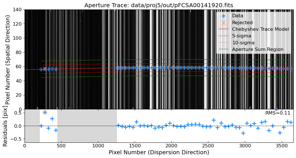
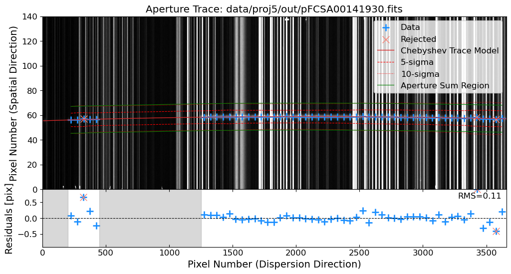
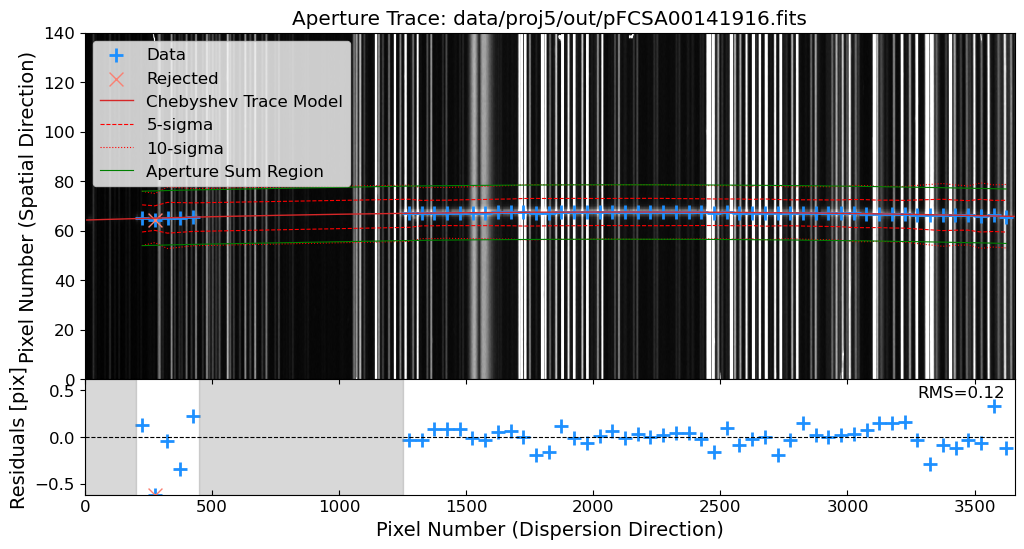
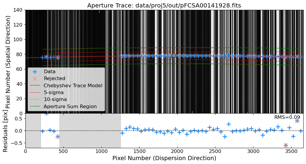
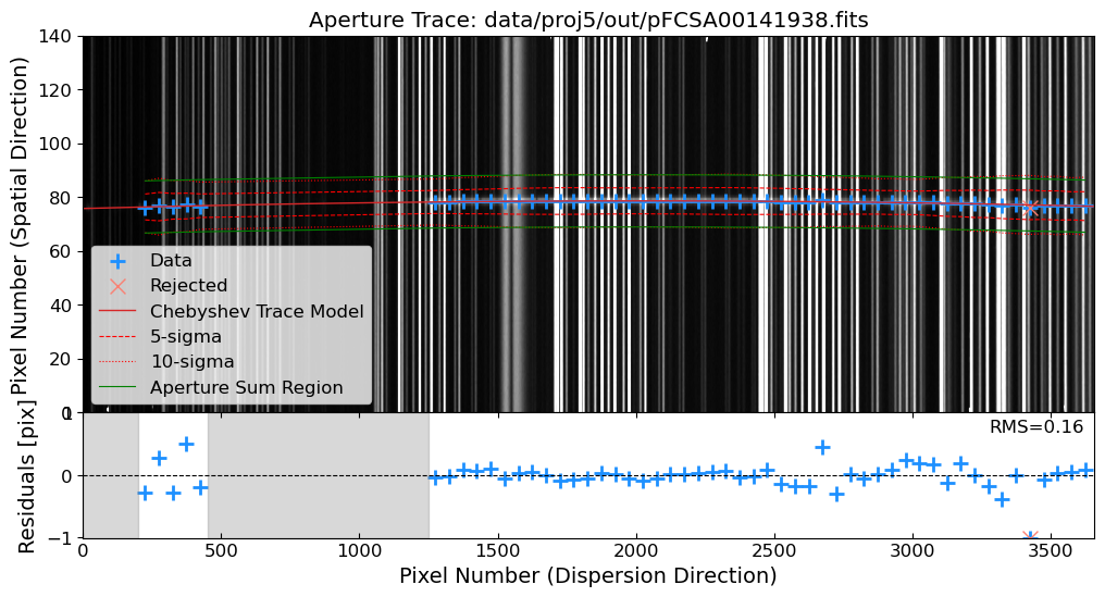
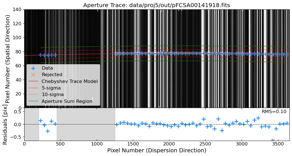
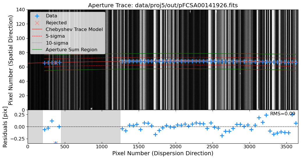
See also

You can also make a interactive plot to see the spatial profile of the source and the background level. You can use the interact function from the ipywidgets module to make an interactive plot. The interact function creates a slider that allows you to change the slice number and see the spatial profile of the source and the background level. This can be useful for identifying the source position and estimating the background level to evaluate the quality of the trace and extraction.

from ipywidgets import interact, IntSlider
image_array = ins.rectified
def plot_vertical_profile(x):
    fig, axes = plt.subplots(1, 2, figsize=(10, 3), gridspec_kw={'width_ratios': [5, 1]})

    # Plotting the image
    ax = axes[0]
    vmin, vmax = interval.get_limits(image_array)
    im = ax.imshow(image_array, cmap='gray', aspect='auto', origin='lower', vmin=vmin, vmax=vmax)
    ax.axvline(x=x, color='red')  # Vertical line at the slider position
    ax.set_title("Image with Vertical Line at Column {}".format(x))
    fig.colorbar(im, label='Intensity')

    # Plotting the vertical profile
    ax = axes[1]
    ax.plot(image_array[:, x], np.arange(image_array.shape[0]), 'r-')
    ax.invert_yaxis()  # Invert y axis to match the image orientation
    ax.set_title("Vertical Profile at Column {}".format(x))
    ax.grid(True)
    ax.set_xlabel('Intensity')
    ax.set_ylabel('Row Index')

    fig.show()
interact(plot_vertical_profile, x=IntSlider(min=0, max=image_array.shape[1]-1, step=1, value=100))

# Plot the extracted spectra
fig = plt.figure(figsize=(12, 4))
ax = fig.add_subplot(111)
ax.set_title("Extracted Spectrum of GRB 130606A")
for SciInsSpec in sci_insspecs:
    ax.plot(SciInsSpec.ap_sum, label=SciInsSpec.fname.stem, lw=0.5, alpha=0.3, c="k")
ax.set_xlabel("Pixel Number (Dispersion Direction)")
ax.set_ylabel("Counts per Exposure Time [e-/s]")
ax.set_ylim(0, 4)

(0.0, 4.0)

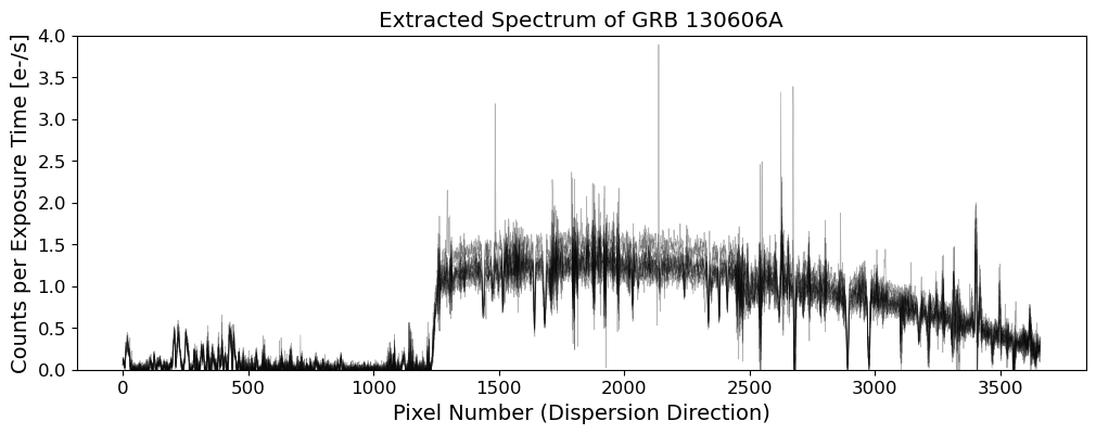
Flux Calibration

The extracted 1D spectra are in counts, which are affected by the instrumental response of the spectrograph. To convert the counts to physical units, such as flux density in erg/s/cm^2/Angstrom, we need to calibrate the flux of the extracted spectra. The flux calibration involves the following steps:

1. Get the Standard Star Spectrum: Obtain the reference spectrum of your standard star from the literature (or observe, calibrate, and make it yourself).

2. Evaluate the Sensitivity Function: Calculate the sensitivity function of the spectrograph, which is the ratio of the observed counts to the true flux of the standard star.

3. Apply the Sensitivity Function: Apply the sensitivity function to the extracted spectra of the science targets to convert the counts to physical units.

The sensitivity function can be calculated by comparing the observed counts of the standard star to the true flux of the standard star. The true flux of the standard star can be obtained from the reference spectrum of the standard star. The sensitivity function is then applied to the extracted spectra of the science targets to convert the counts to physical units.

In this case, we need to obtain the reference spectrum of Feige 34. The reference spectrum of Feige 34 can be obtained from the STScI CALSPEC database. This file is also available in the feige34_stis_004.fits file in our repository.

# reference spectrum
stdref = Table.read(WD / "feige34_stis_004.fits")
stdref_wave = stdref["WAVELENGTH"].value
stdref_flux = stdref["FLUX"].value

# observed spectrum in instrumental units
stdinst_flux = np.mean(
    [std_insspecs[i].ap_sum for i in range(len(std_insspecs))], axis=0
)
stdinst_wave = wavegrid

# resample the reference spectrum using flux-conserving method
input_spectra = Spectrum1D(
    spectral_axis=stdref_wave * u.AA, flux=stdref_flux * u.erg / u.s / u.cm**2 / u.AA
)
fluxc_resample = FluxConservingResampler()
stdref_resampled = fluxc_resample(input_spectra, stdinst_wave * u.AA)
stdref_flux_resampled = stdref_resampled.flux.value

WARNING: UnitsWarning: 'ANGSTROMS' did not parse as fits unit: At col 0, Unit 'ANGSTROMS' not supported by the FITS standard. Did you mean Angstrom or angstrom? If this is meant to be a custom unit, define it with 'u.def_unit'. To have it recognized inside a file reader or other code, enable it with 'u.add_enabled_units'. For details, see https://docs.astropy.org/en/latest/units/combining_and_defining.html [astropy.units.core]
WARNING: UnitsWarning: 'FLAM' did not parse as fits unit: At col 0, Unit 'FLAM' not supported by the FITS standard. Did you mean flm? If this is meant to be a custom unit, define it with 'u.def_unit'. To have it recognized inside a file reader or other code, enable it with 'u.add_enabled_units'. For details, see https://docs.astropy.org/en/latest/units/combining_and_defining.html [astropy.units.core]
WARNING: UnitsWarning: 'NONE' did not parse as fits unit: At col 0, Unit 'NONE' not supported by the FITS standard.  If this is meant to be a custom unit, define it with 'u.def_unit'. To have it recognized inside a file reader or other code, enable it with 'u.add_enabled_units'. For details, see https://docs.astropy.org/en/latest/units/combining_and_defining.html [astropy.units.core]
WARNING: UnitsWarning: 'SEC' did not parse as fits unit: At col 0, Unit 'SEC' not supported by the FITS standard. Did you mean EC? If this is meant to be a custom unit, define it with 'u.def_unit'. To have it recognized inside a file reader or other code, enable it with 'u.add_enabled_units'. For details, see https://docs.astropy.org/en/latest/units/combining_and_defining.html [astropy.units.core]

# setting masking regions
masking_windows = [[7560, 7730], [8120, 8400], [8930, 9700], [10010, 10150]]

fig = plt.figure(figsize=(12, 4))
ax1 = fig.add_subplot(121)
ax1.plot(stdinst_wave, stdinst_flux, c="k", lw=0.8)
ax1.set_title("Feige34 Instrumental Spectrum")
ax1.set_xlabel("Wavelength [Å]")
ax1.set_ylabel("Counts per Exposure Time [e-/s]")
xlim = ax1.get_xlim()
ax2 = fig.add_subplot(122)
ax2.plot(
    stdinst_wave,
    stdref_flux_resampled,
    c="tab:blue",
    lw=0.8,
    label="Resampled",
    zorder=2,
)
ylim = ax2.get_ylim()
ax2.plot(stdref_wave, stdref_flux, c="k", lw=0.8, label="Original")
ax2.set_title("Feige34 Reference Spectrum")
ax2.set_xlabel("Wavelength [Å]")
ax2.set_ylabel("Flux [erg/s/cm²/Å]")
ax2.set_xlim(xlim)
ax2.set_ylim(ylim)
ax2.legend()

for ax in [ax1, ax2]:
    for window in masking_windows:
        ax.axvspan(window[0], window[1], color="gray", alpha=0.1, zorder=1)

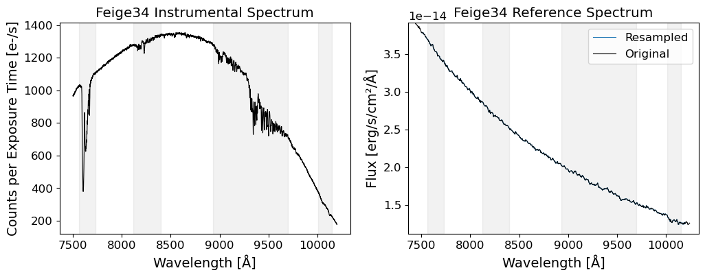
# polynomial fitting
order_sensfunc = 9

ratio = stdref_flux_resampled / stdinst_flux
mask = np.zeros_like(stdinst_wave, dtype=bool)
for window in masking_windows:
    mask |= (stdinst_wave > window[0]) & (stdinst_wave < window[1])

# fitting the sensitivity function in logarithmic scale
logratio = np.log10(ratio)

coeffs = np.polyfit(stdinst_wave[~mask], logratio[~mask], order_sensfunc)
logsensfunc = np.polyval(coeffs, stdinst_wave)
sensfunc = 10**logsensfunc

# plot the sensitivity function
fig = plt.figure(figsize=(12, 4))
ax = fig.add_subplot(111)
ax.scatter(stdinst_wave, ratio, c="tab:blue", s=2, marker="+", label="Ratio")
ax.plot(stdinst_wave, sensfunc, c="tab:red", lw=0.8, label="Model Sensitivity Function")
ax.set_title("Sensitivity Function")
ax.set_xlabel("Wavelength [Å]")
ax.set_ylabel("Sensitivity [erg/s/cm²/Å/(e-/s)]")
for window in masking_windows:
    ax.axvspan(window[0], window[1], color="gray", alpha=0.1)

ax.legend()

/opt/anaconda3/envs/main/lib/python3.11/site-packages/IPython/core/interactiveshell.py:3577: RankWarning:

Polyfit may be poorly conditioned

<matplotlib.legend.Legend at 0x1f4e25950>

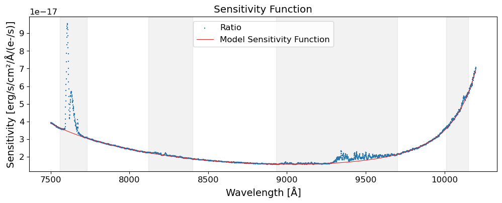
# apply the sensitivity function to the observed spectra
fig = plt.figure(figsize=(12, 4))
ax1 = fig.add_subplot(121)
ax1.plot(stdinst_wave, stdinst_flux * sensfunc, c="k", lw=0.8)
ax1.set_title("Feige34 Standardized Spectrum")
ax1.set_xlabel("Wavelength [Å]")
ax1.set_ylabel("Flux [erg/s/cm²/Å]")
xlim = ax1.get_xlim()
ax2 = fig.add_subplot(122)
ax2.plot(
    stdinst_wave,
    stdref_flux_resampled,
    c="tab:blue",
    lw=0.8,
    label="Resampled",
    zorder=2,
)
ylim = ax2.get_ylim()
ax2.plot(stdref_wave, stdref_flux, c="k", lw=0.8, label="Original")
ax2.set_title("Feige34 Reference Spectrum")
ax2.set_xlabel("Wavelength [Å]")
ax2.set_ylabel("Flux [erg/s/cm²/Å]")
ax2.set_xlim(xlim)
ax2.set_ylim(ylim)
ax2.legend()

for ax in [ax1, ax2]:
    for window in masking_windows:
        ax.axvspan(window[0], window[1], color="gray", alpha=0.1, zorder=1)

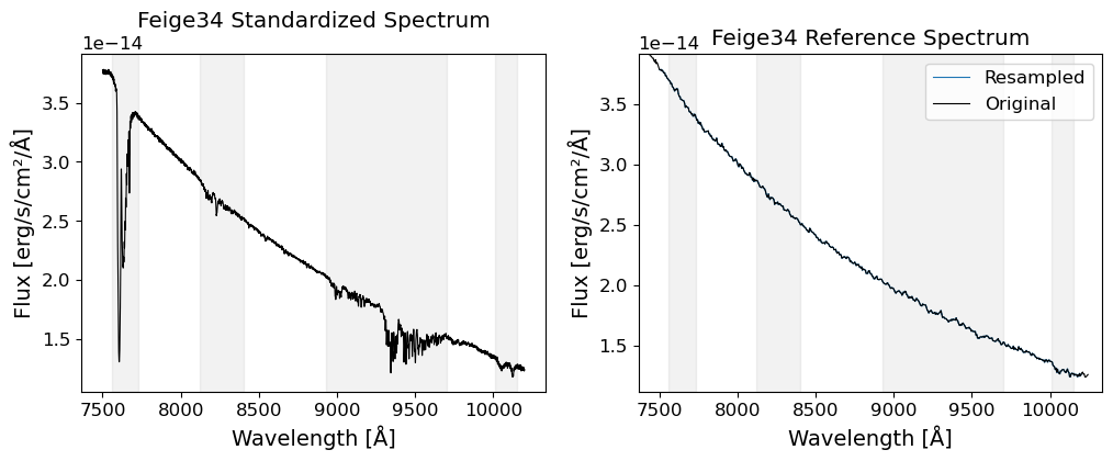
# save the sensitivity function
sensfunc_table = Table([stdinst_wave, sensfunc], names=["WAVELENGTH", "SENSFUNC"])
sensfunc_table.write(OUTDIR / "sensfunc.fits", overwrite=True)

# apply the sensitivity function to the science spectra
for ins in sci_insspecs:
    ins.flux = ins.ap_sum * sensfunc
    ins.fluxerr = ins.ap_sig * sensfunc

# plot the standardized science spectra
fig = go.Figure()
for ins in sci_insspecs:
    fig.add_trace(
        go.Scatter(
            x=wavegrid,
            y=ins.flux,
            error_y=dict(
                type="data",
                array=ins.fluxerr,
                visible=True,
                thickness=1,
                width=1,
            ),
            mode="lines+markers",
            marker=dict(size=3),
            line=dict(width=0.8),
            name=ins.fname.stem,
        )
    )

fig.update_layout(
    title="Standardized Science Spectra",
    xaxis_title="Wavelength [Å]",
    yaxis_title="Flux [erg/s/cm²/Å]",
    showlegend=True,
    legend=dict(yanchor="top", y=0.99, xanchor="left", x=0.01),
)
fig

References

• Totani et al. (2014)