Concept of spectroscopy#
Author: Jooyeon Geem, Hyeonguk Bahk
%config InlineBackend.figure_format = 'retina'
# %matplotlib widget
# %matplotlib notebook
import numpy as np
import os
import glob
from pathlib import Path
from matplotlib import pyplot as plt
from astropy.io import ascii, fits
from astropy.table import Table,Column
from datetime import datetime
from scipy.optimize import curve_fit
from scipy.ndimage import median_filter
from scipy.interpolate import UnivariateSpline
from mpl_toolkits.axes_grid1 import make_axes_locatable
from skimage.feature import peak_local_max
from astropy.stats import sigma_clip, gaussian_fwhm_to_sigma
from numpy.polynomial.chebyshev import chebfit, chebval
from astropy.modeling.models import Gaussian1D, Chebyshev2D
from astropy.modeling.fitting import LevMarLSQFitter
from matplotlib import gridspec, rcParams, rc
from IPython.display import Image

plt.rcParams['axes.linewidth'] = 2
plt.rcParams['font.size'] = 10
plt.rcParams['xtick.labelsize'] = 15
plt.rcParams['ytick.labelsize'] = 15
# Define your working directory
HOME = Path.home()
WD = HOME/'class'/'ao22'/'SNU_AO22-2'/'_test'
SUBPATH = WD/'data'

Biaslist = sorted(list(Path.glob(SUBPATH, 'calibration*bias.fit')))

Darklist= sorted(list(Path.glob(SUBPATH, 'calibration*dk*.fit')))

Flatlist = sorted(list(Path.glob(SUBPATH, 'Flat*.fit')))

Complist = sorted(list(Path.glob(SUBPATH, 'Neon*L.fit')))

Objectlist = sorted(list(Path.glob(SUBPATH, '61Cygni*.fit')))

Standlist = sorted(list(Path.glob(SUBPATH, 'HR153*.fit')))

# Checking the paths
print(Table([Biaslist], names=['Bias']), 2*'\n')
print(Table([Darklist], names=['Darklist']), 2*'\n')
print(Table([Flatlist], names=['Flatlist']), 2*'\n')
print(Table([Complist], names=['Complist']), 2*'\n')
print(Table([Objectlist], names=['Objectlist']), 2*'\n')
print(Table([Standlist], names=['Standlist']), 2*'\n')
                                 Bias
----------------------------------------------------------------------
/Users/hbahk/class/ao22/SNU_AO22-2/_test/data/calibration-0001bias.fit
/Users/hbahk/class/ao22/SNU_AO22-2/_test/data/calibration-0002bias.fit
/Users/hbahk/class/ao22/SNU_AO22-2/_test/data/calibration-0003bias.fit
/Users/hbahk/class/ao22/SNU_AO22-2/_test/data/calibration-0004bias.fit
/Users/hbahk/class/ao22/SNU_AO22-2/_test/data/calibration-0005bias.fit
/Users/hbahk/class/ao22/SNU_AO22-2/_test/data/calibration-0006bias.fit
/Users/hbahk/class/ao22/SNU_AO22-2/_test/data/calibration-0007bias.fit
/Users/hbahk/class/ao22/SNU_AO22-2/_test/data/calibration-0008bias.fit
/Users/hbahk/class/ao22/SNU_AO22-2/_test/data/calibration-0009bias.fit


                               Darklist
----------------------------------------------------------------------
 /Users/hbahk/class/ao22/SNU_AO22-2/_test/data/calibration-0001dk1.fit
/Users/hbahk/class/ao22/SNU_AO22-2/_test/data/calibration-0001dk10.fit
 /Users/hbahk/class/ao22/SNU_AO22-2/_test/data/calibration-0001dk2.fit
/Users/hbahk/class/ao22/SNU_AO22-2/_test/data/calibration-0001dk60.fit
 /Users/hbahk/class/ao22/SNU_AO22-2/_test/data/calibration-0002dk1.fit
/Users/hbahk/class/ao22/SNU_AO22-2/_test/data/calibration-0002dk10.fit
 /Users/hbahk/class/ao22/SNU_AO22-2/_test/data/calibration-0002dk2.fit
/Users/hbahk/class/ao22/SNU_AO22-2/_test/data/calibration-0002dk60.fit
 /Users/hbahk/class/ao22/SNU_AO22-2/_test/data/calibration-0003dk1.fit
/Users/hbahk/class/ao22/SNU_AO22-2/_test/data/calibration-0003dk10.fit
 /Users/hbahk/class/ao22/SNU_AO22-2/_test/data/calibration-0003dk2.fit
/Users/hbahk/class/ao22/SNU_AO22-2/_test/data/calibration-0003dk60.fit
 /Users/hbahk/class/ao22/SNU_AO22-2/_test/data/calibration-0004dk1.fit
/Users/hbahk/class/ao22/SNU_AO22-2/_test/data/calibration-0004dk10.fit
 /Users/hbahk/class/ao22/SNU_AO22-2/_test/data/calibration-0004dk2.fit
/Users/hbahk/class/ao22/SNU_AO22-2/_test/data/calibration-0004dk60.fit
 /Users/hbahk/class/ao22/SNU_AO22-2/_test/data/calibration-0005dk1.fit
/Users/hbahk/class/ao22/SNU_AO22-2/_test/data/calibration-0005dk10.fit
 /Users/hbahk/class/ao22/SNU_AO22-2/_test/data/calibration-0005dk2.fit
/Users/hbahk/class/ao22/SNU_AO22-2/_test/data/calibration-0005dk60.fit
 /Users/hbahk/class/ao22/SNU_AO22-2/_test/data/calibration-0006dk1.fit
/Users/hbahk/class/ao22/SNU_AO22-2/_test/data/calibration-0006dk10.fit
 /Users/hbahk/class/ao22/SNU_AO22-2/_test/data/calibration-0006dk2.fit
/Users/hbahk/class/ao22/SNU_AO22-2/_test/data/calibration-0006dk60.fit
 /Users/hbahk/class/ao22/SNU_AO22-2/_test/data/calibration-0007dk1.fit
/Users/hbahk/class/ao22/SNU_AO22-2/_test/data/calibration-0007dk10.fit
 /Users/hbahk/class/ao22/SNU_AO22-2/_test/data/calibration-0007dk2.fit
/Users/hbahk/class/ao22/SNU_AO22-2/_test/data/calibration-0007dk60.fit
 /Users/hbahk/class/ao22/SNU_AO22-2/_test/data/calibration-0008dk1.fit
/Users/hbahk/class/ao22/SNU_AO22-2/_test/data/calibration-0008dk10.fit
 /Users/hbahk/class/ao22/SNU_AO22-2/_test/data/calibration-0008dk2.fit
/Users/hbahk/class/ao22/SNU_AO22-2/_test/data/calibration-0008dk60.fit
 /Users/hbahk/class/ao22/SNU_AO22-2/_test/data/calibration-0009dk1.fit
/Users/hbahk/class/ao22/SNU_AO22-2/_test/data/calibration-0009dk10.fit
 /Users/hbahk/class/ao22/SNU_AO22-2/_test/data/calibration-0009dk2.fit
/Users/hbahk/class/ao22/SNU_AO22-2/_test/data/calibration-0009dk60.fit


                          Flatlist
-----------------------------------------------------------
/Users/hbahk/class/ao22/SNU_AO22-2/_test/data/Flat-0001.fit
/Users/hbahk/class/ao22/SNU_AO22-2/_test/data/Flat-0002.fit
/Users/hbahk/class/ao22/SNU_AO22-2/_test/data/Flat-0003.fit
/Users/hbahk/class/ao22/SNU_AO22-2/_test/data/Flat-0004.fit
/Users/hbahk/class/ao22/SNU_AO22-2/_test/data/Flat-0005.fit
/Users/hbahk/class/ao22/SNU_AO22-2/_test/data/Flat-0006.fit
/Users/hbahk/class/ao22/SNU_AO22-2/_test/data/Flat-0007.fit
/Users/hbahk/class/ao22/SNU_AO22-2/_test/data/Flat-0008.fit
/Users/hbahk/class/ao22/SNU_AO22-2/_test/data/Flat-0009.fit


                          Complist
------------------------------------------------------------
/Users/hbahk/class/ao22/SNU_AO22-2/_test/data/Neon-0001L.fit
/Users/hbahk/class/ao22/SNU_AO22-2/_test/data/Neon-0002L.fit
/Users/hbahk/class/ao22/SNU_AO22-2/_test/data/Neon-0003L.fit
/Users/hbahk/class/ao22/SNU_AO22-2/_test/data/Neon-0004L.fit
/Users/hbahk/class/ao22/SNU_AO22-2/_test/data/Neon-0005L.fit


                          Objectlist
--------------------------------------------------------------
/Users/hbahk/class/ao22/SNU_AO22-2/_test/data/61Cygni-0001.fit
/Users/hbahk/class/ao22/SNU_AO22-2/_test/data/61Cygni-0002.fit
/Users/hbahk/class/ao22/SNU_AO22-2/_test/data/61Cygni-0003.fit
/Users/hbahk/class/ao22/SNU_AO22-2/_test/data/61Cygni-0004.fit
/Users/hbahk/class/ao22/SNU_AO22-2/_test/data/61Cygni-0005.fit


                         Standlist
------------------------------------------------------------
/Users/hbahk/class/ao22/SNU_AO22-2/_test/data/HR153-0001.fit
/Users/hbahk/class/ao22/SNU_AO22-2/_test/data/HR153-0002.fit
/Users/hbahk/class/ao22/SNU_AO22-2/_test/data/HR153-0003.fit
/Users/hbahk/class/ao22/SNU_AO22-2/_test/data/HR153-0004.fit
/Users/hbahk/class/ao22/SNU_AO22-2/_test/data/HR153-0005.fit
1. Preprocessing (i.e., Bias subtraction, Dark subtraction, Flat fielding)#
1.1 Making master bias#
Before making master bias, we have to check whethere there is a peculiar bias image.
# Checking the bias image
Name = []
Mean = []
Min = []
Max = []
Std = []

for i in range(len(Biaslist)):
    hdul = fits.open(Biaslist[i])
    data = hdul[0].data
    data = np.array(data).astype('float64')  # Change datatype from uint16 to float64
    mean = np.mean(data)
    minimum = np.min(data)
    maximum = np.max(data)
    stdev = np.std(data)
    print(Biaslist[i],mean,minimum,maximum)

    Name.append(os.path.basename(Biaslist[i]))
    Mean.append("%.2f" % mean )
    Min.append("%.2f" % minimum)
    Max.append("{0:.2f}".format(maximum))
    Std.append(f'{stdev:.2f}')

table = Table([Name, Mean, Min, Max, Std],
              names=['Filename','Mean','Min','Max','Std'])
print(table)
/Users/hbahk/class/ao22/SNU_AO22-2/_test/data/calibration-0001bias.fit 152.78639256198346 111.0 190.0
/Users/hbahk/class/ao22/SNU_AO22-2/_test/data/calibration-0002bias.fit 152.8369297520661 121.0 198.0
/Users/hbahk/class/ao22/SNU_AO22-2/_test/data/calibration-0003bias.fit 152.9803347107438 118.0 188.0
/Users/hbahk/class/ao22/SNU_AO22-2/_test/data/calibration-0004bias.fit 152.98019008264464 116.0 193.0
/Users/hbahk/class/ao22/SNU_AO22-2/_test/data/calibration-0005bias.fit 152.91122727272727 112.0 191.0
/Users/hbahk/class/ao22/SNU_AO22-2/_test/data/calibration-0006bias.fit 152.86499586776858 114.0 191.0
/Users/hbahk/class/ao22/SNU_AO22-2/_test/data/calibration-0007bias.fit 152.9045123966942 118.0 196.0
/Users/hbahk/class/ao22/SNU_AO22-2/_test/data/calibration-0008bias.fit 152.873347107438 118.0 189.0
/Users/hbahk/class/ao22/SNU_AO22-2/_test/data/calibration-0009bias.fit 152.9414173553719 121.0 193.0
        Filename          Mean   Min    Max   Std
------------------------ ------ ------ ------ ----
calibration-0001bias.fit 152.79 111.00 190.00 4.80
calibration-0002bias.fit 152.84 121.00 198.00 4.80
calibration-0003bias.fit 152.98 118.00 188.00 4.78
calibration-0004bias.fit 152.98 116.00 193.00 4.80
calibration-0005bias.fit 152.91 112.00 191.00 4.83
calibration-0006bias.fit 152.86 114.00 191.00 4.80
calibration-0007bias.fit 152.90 118.00 196.00 4.81
calibration-0008bias.fit 152.87 118.00 189.00 4.82
calibration-0009bias.fit 152.94 121.00 193.00 4.79
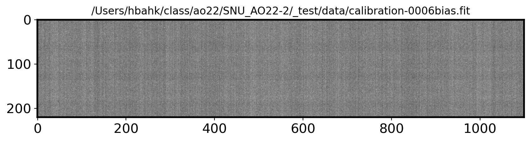
# Plot the Sample image of bias image
File = Biaslist[5]  # pick one of the bias image
sample_hdul = fits.open(File)
sample_data = sample_hdul[0].data

fig,ax = plt.subplots(1,1,figsize=(10,5))
vmin = np.mean(sample_data) - 40
vmax = np.mean(sample_data) + 40
im = ax.imshow(sample_data,
               cmap='gray', vmin=vmin, vmax=vmax)
ax.set_title(File, fontsize=12)
Text(0.5, 1.0, '/Users/hbahk/class/ao22/SNU_AO22-2/_test/data/calibration-0006bias.fit')
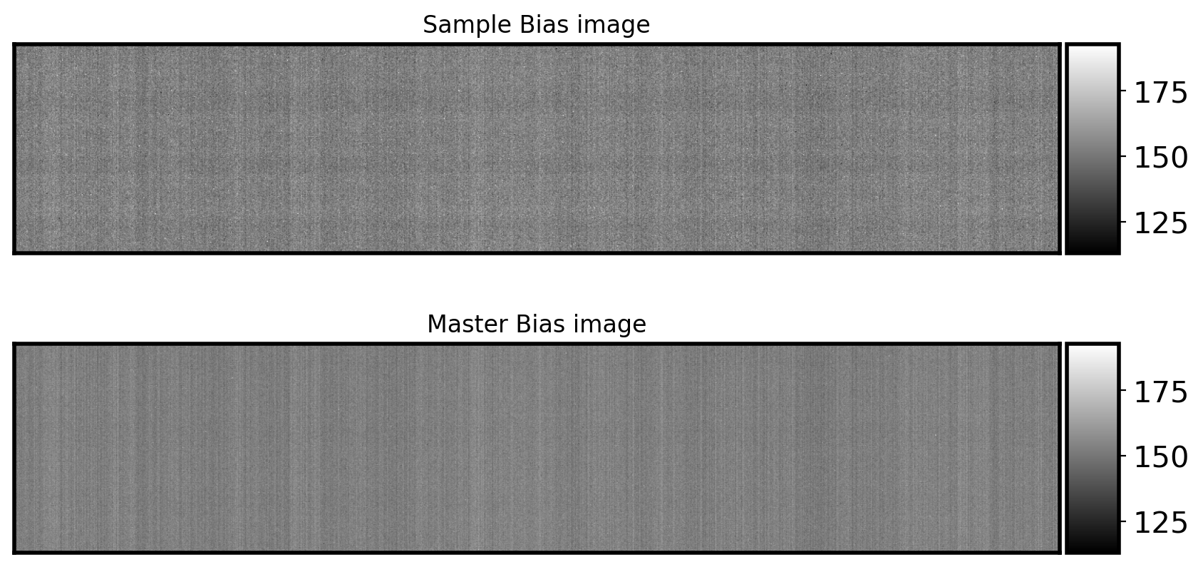
# Median combine Bias image

Master_bias = []
for i in range(0,len(Biaslist)):
    hdul = fits.open(Biaslist[i])
    bias_data = hdul[0].data
    bias_data = np.array(bias_data).astype('float64')
    Master_bias.append(bias_data)
MASTER_Bias = np.median(Master_bias,axis=0)


# Let's make Master bias image fits file

# Making header part
bias_header = hdul[0].header  # fetch header from one of bias images
bias_header['OBJECT'] = 'Bias'
# - add information about the combine process to header comment
bias_header['COMMENT'] = f'{Biaslist} bias images are median combined on ' \
                          + datetime.now().strftime('%Y-%m-%d %H:%M:%S (KST)')


SAVE_bias = SUBPATH/'Master_Bias.fits'  # path to save master bias
fits.writeto(SAVE_bias, MASTER_Bias, header=bias_header, overwrite=True)


# Plot Master bias
fig,ax = plt.subplots(2, 1, figsize=(10,5))
im = ax[0].imshow(sample_data, cmap='gray',
                  vmin=vmin, vmax=vmax)
divider = make_axes_locatable(ax[0])
cax = divider.append_axes("right", size="5%", pad=0.05)
ax[0].set_title('Sample Bias image')
ax[0].tick_params(labelbottom=False, labelleft=False,
                  bottom=False, left=False)
plt.colorbar(im,cax=cax)

im1 = ax[1].imshow(MASTER_Bias, cmap='gray',
                   vmin=vmin, vmax=vmax)
divider = make_axes_locatable(ax[1])
cax = divider.append_axes("right", size='5%', pad=0.05)
ax[1].set_title('Master Bias image')
ax[1].tick_params(labelbottom=False, labelleft=False,
                  bottom=False, left=False)
plt.colorbar(im1, cax=cax)
<matplotlib.colorbar.Colorbar at 0x7f9578140520>
1.2 Derive Readout Noise (RN)#
# Let's derive RN

# The following is just to give you an idea about the calculation
# - Bring Bias1 data
hdul1 = fits.open(Biaslist[0])
bias1 = hdul1[0].data
bias1 = np.array(bias1).astype('float64')

# - Bring Bias2 data
hdul2 = fits.open(Biaslist[1])
bias2 = hdul2[0].data
bias2 = np.array(bias2).astype('float64')

# - Derive the differential image
dbias = bias2 - bias1

# - Bring Gain
gain = 1.5 #e/ADU

# - Calculate RN
RN = np.std(dbias)*gain / np.sqrt(2)
print(f'Readout Noise is {RN:.2f}')


# Let's do it for all bias data
Name = []
RN = []
for i in range(len(Biaslist)-1):
    hdul1 = fits.open(Biaslist[i])
    bias1 = hdul1[0].data
    bias1 = np.array(bias1).astype('float64')
    hdul2 = fits.open(Biaslist[i+1])
    bias2 = hdul2[0].data
    bias2 = np.array(bias2).astype('float64')
    dbias = bias2 - bias1

    print(i,'st',np.std(dbias)*gain / np.sqrt(2))
    RN.append(np.std(dbias)*gain / np.sqrt(2))
print('\nmean RN:', np.mean(RN))
RN = np.mean(RN)
Readout Noise is 6.33
0 st 6.327328539930154
1 st 6.340204240265304
2 st 6.339680597614822
3 st 6.341643681666518
4 st 6.360511037222893
5 st 6.351511335524966
6 st 6.344696431761455
7 st 6.364776809710108

mean RN: 6.346294084212028
1.3 Making Master Dark#
Master dark = median combine([Dark image1 - master bias, Dark image2 - master bias, Dark image3 - master bias,…])
# Checking what exposure time is taken
exptime = []

for i in range(len(Darklist)):
    hdul = fits.open(Darklist[i])[0]
    header = hdul.header
    exp = header['EXPTIME']  # get exposure time from its header
    exptime.append(exp)
exptime = set(exptime)  # only unique elements will be remained
exptime = sorted(exptime)
print(exptime)
[1.0, 2.0, 10.0, 60.0]
# Bring master bias
Mbias = fits.open(SAVE_bias)[0].data
Mbias = np.array(Mbias).astype('float64')

# Making master dark image for each exposure time
for exp_i in exptime:
    Master_dark = []
    for i in range(len(Darklist)):
        hdul = fits.open(Darklist[i])[0]
        header = hdul.header
        exp = header['EXPTIME']

        if exp == exp_i:
            data = hdul.data
            data = np.array(data).astype('float64')
            bdata = data - Mbias  # bias subtracting
            Master_dark.append(bdata)

    MASTER_dark = np.median(Master_dark, axis=0)  # median combine bias-subtracted dark frames

    header['COMMENT'] = 'Bias_subtraction is done' + datetime.now().strftime('%Y-%m-%d %H:%M:%S (KST)')
    header["COMMENT"] = f'{len(Master_dark)} dark images are median combined on '\
                         + datetime.now().strftime('%Y-%m-%d %H:%M:%S (KST)')

    SAVE_dark = SUBPATH/('Master_Dark_'+str(exp_i)+'s.fits')
    fits.writeto(SAVE_dark, MASTER_dark, header=header, overwrite=True)
    print(exp_i ,'s is done!', SAVE_dark,' is made.')
1.0 s is done! /Users/hbahk/class/ao22/SNU_AO22-2/_test/data/Master_Dark_1.0s.fits  is made.
2.0 s is done! /Users/hbahk/class/ao22/SNU_AO22-2/_test/data/Master_Dark_2.0s.fits  is made.
10.0 s is done! /Users/hbahk/class/ao22/SNU_AO22-2/_test/data/Master_Dark_10.0s.fits  is made.
60.0 s is done! /Users/hbahk/class/ao22/SNU_AO22-2/_test/data/Master_Dark_60.0s.fits  is made.
1.4 Making Master Flat#
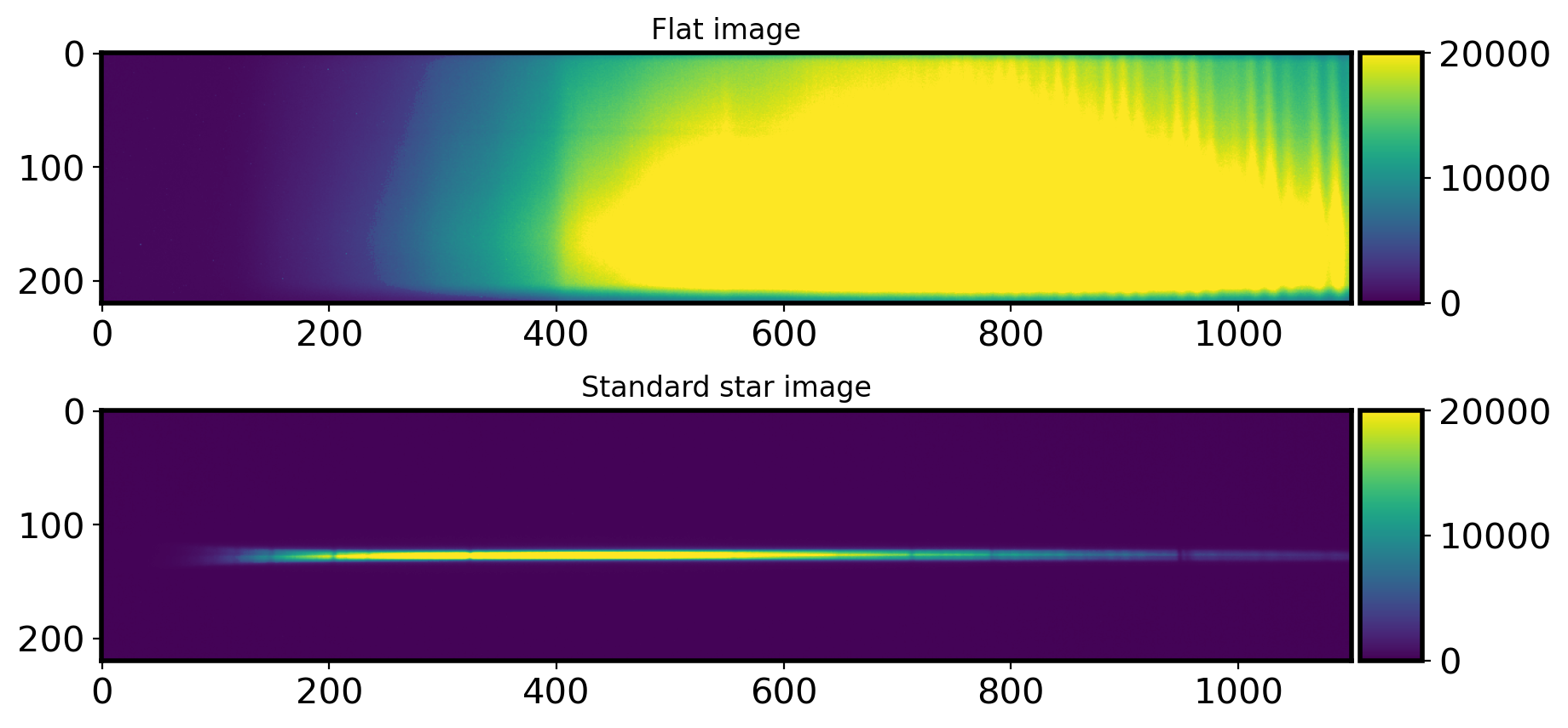
1.4-1 Checking whether Flat image is shifted or not#
The flat image could shift little by little depending on where the telescope is pointing. Because different images may have different flats to use, it can be dangerous to median combine all the flats image taken overnight. Let’s do quick and rough check whethere there is flat shift.
By using local peak location, I will check whether there was the flat shift or not.
# Plot the flat image
fig, ax = plt.subplots(2, 1, figsize=(10, 5))
hdul = fits.open(Flatlist[4])[0]
data = hdul.data
im = ax[0].imshow(data, vmin=0, vmax=20000)
ax[0].set_title('Flat image')
divider = make_axes_locatable(ax[0])
cax = divider.append_axes("right" ,size='5%', pad=0.05)
plt.colorbar(im, cax=cax)

# Standard star image
hdul = fits.open(Standlist[0])[0]
data = hdul.data
im = ax[1].imshow(data, vmin=0, vmax=20000)
ax[1].set_title('Standard star image')
divider = make_axes_locatable(ax[1])
cax = divider.append_axes("right" ,size='5%', pad=0.05)
plt.colorbar(im, cax=cax)
<matplotlib.colorbar.Colorbar at 0x7f95aafac460>
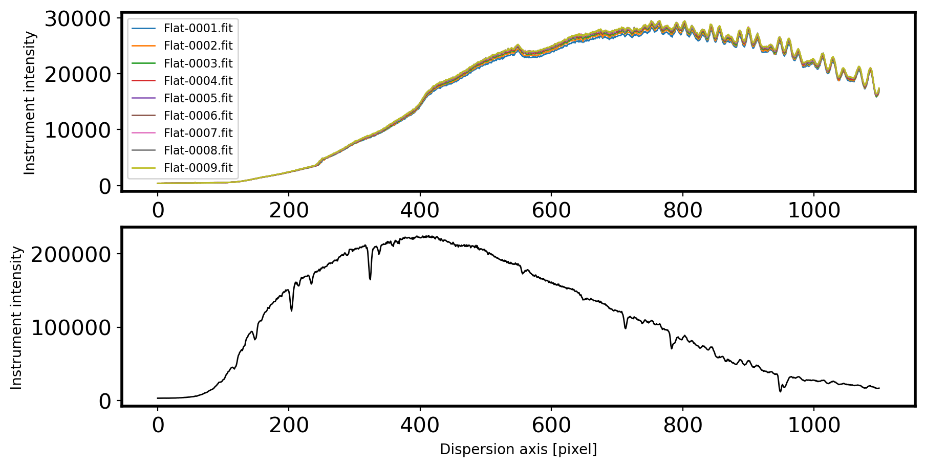
# Checking intensity profile through the dispersion axis

fig,ax = plt.subplots(2,1,figsize=(10,5))

for i in range(len(Flatlist)):
    hdul = fits.open(Flatlist[i])[0]
    data = hdul.data.astype('float64')
    flat = np.mean(data[115:135,:], axis=0)

    ax[0].plot(flat, label=Flatlist[i].name, lw=1)
    ax[0].legend(fontsize=8)
    ax[0].set_ylabel('Instrument intensity')
    ax[0].set_xlabel('Dispersion axis [pixel]')

hdul_std = fits.open(Standlist[0])[0]
data_std = hdul_std.data.astype('float64')
std = np.sum(data_std[115:135,:], axis=0)
ax[1].plot(std, label=Standlist[0].name, lw=1, c='k')
ax[1].set_ylabel('Instrument intensity')
ax[1].set_xlabel('Dispersion axis [pixel]')
Text(0.5, 0, 'Dispersion axis [pixel]')
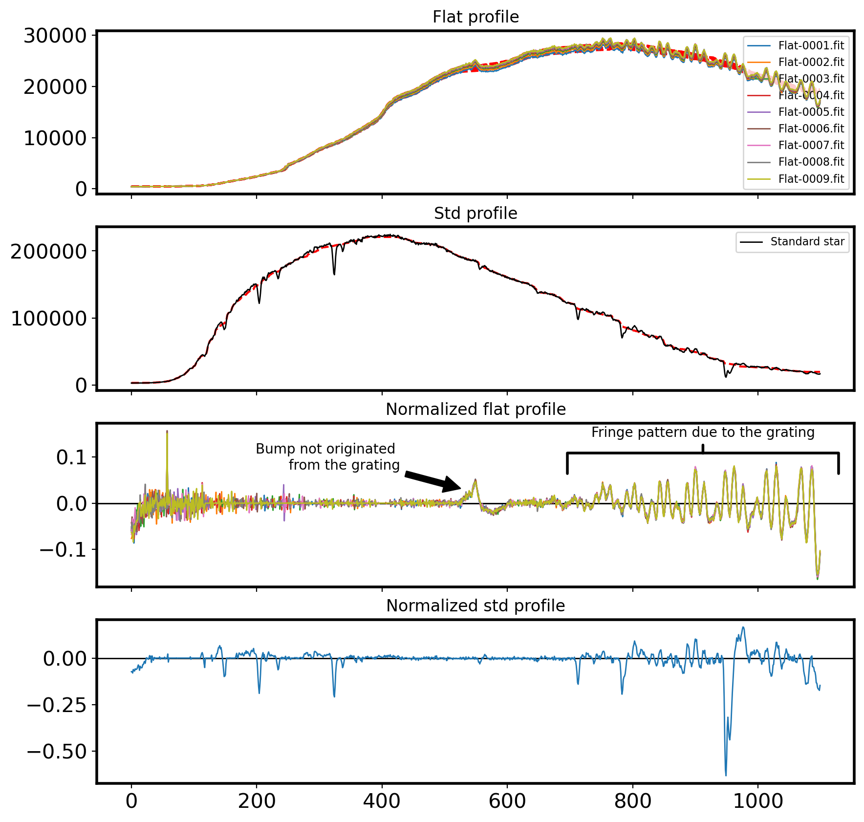
Comparing with the Standard Star Profile#
The above flat spectra shows many wiggles and bumps. Yet, we don’t know if these features are originated from the grating, which in turn will affect our science frame equally. If they are not due to the grating, such as filters in front of the flat-field lamp, the extreme difference in color temperature between the lamps and the object of interest, or wavelength-dependent variations in the reflectivity of the paint used for the flat-field screen (Massey & Hansen, 2010), they are not going to present on the science frame.
Let’s see if a supposedly smooth source (in this case, a standard star) has same “wiggles” and “bumps” on its spectrum. If this is the case, we should model the flat lamp with “high order” and normalize the flat image with this model. If not, we should adopt “low-order” model or constant to normalize our flat field.
fig,ax = plt.subplots(4,1,figsize=(10,10), sharex=True)

def smooth(y, width):    # Moving box averaging
    box = np.ones(width)/width
    y_smooth = np.convolve(y, box, mode='same')
    return y_smooth

smoothing_size = 100
smoother = median_filter

Coor_shift = []
for i in range(len(Flatlist)):
    hdul = fits.open(Flatlist[i])[0]
    data = hdul.data.astype('float64')
    flat = np.mean(data[115:135,:], axis=0)

    ax[0].plot(flat,label=Flatlist[i].name, lw=1, zorder=20)
    ax[0].legend(fontsize=8)

    sflat = smoother(flat, smoothing_size)
    nor_flat = flat/sflat  # flat field normalized by smoothed curve
    ax[0].plot(sflat, color='r', ls='--')

    ax[2].plot((flat-sflat)/sflat, lw=1, zorder=15, label=Flatlist[i].name)
    # ax[2].legend(fontsize=8)
    ax[2].axhline(0, color='k', lw=1)

# Let's see if a supposedly smooth source (in this case, a standard star)
# has same "wiggles" and "bumps" on its spectrum. If this is the case, we should
# model the flat lamp with "high order" and normalize the flat image with the model.
# If not, we
sstd = smoother(std, smoothing_size)

ax[1].plot(std,label='Standard star', c='k', lw=1, zorder=20)
ax[1].plot(sstd, color='r', ls='--')
ax[1].legend(fontsize=8)

ax[3].plot((std-sstd)/sstd, lw=1, zorder=15)
ax[3].axhline(0, color='k', lw=1)

ax[2].annotate('Fringe pattern due to the grating', xy=(0.8, 0.8), xytext=(0.8, 0.9), xycoords='axes fraction',
               ha='center', va='bottom',
               arrowprops=dict(arrowstyle='-[, widthB=10.0, lengthB=1.5', lw=2.0))
ax[2].annotate('Bump not originated \n from the grating', xy=(530, 0.03),  xycoords='data',
               xytext=(0.4, 0.7), textcoords='axes fraction',
               arrowprops=dict(facecolor='black', shrink=0.05),
               ha='right', va='bottom')

ax[0].set_title('Flat profile')
ax[1].set_title('Std profile')
ax[2].set_title('Normalized flat profile')
ax[3].set_title('Normalized std profile')
Text(0.5, 1.0, 'Normalized std profile')
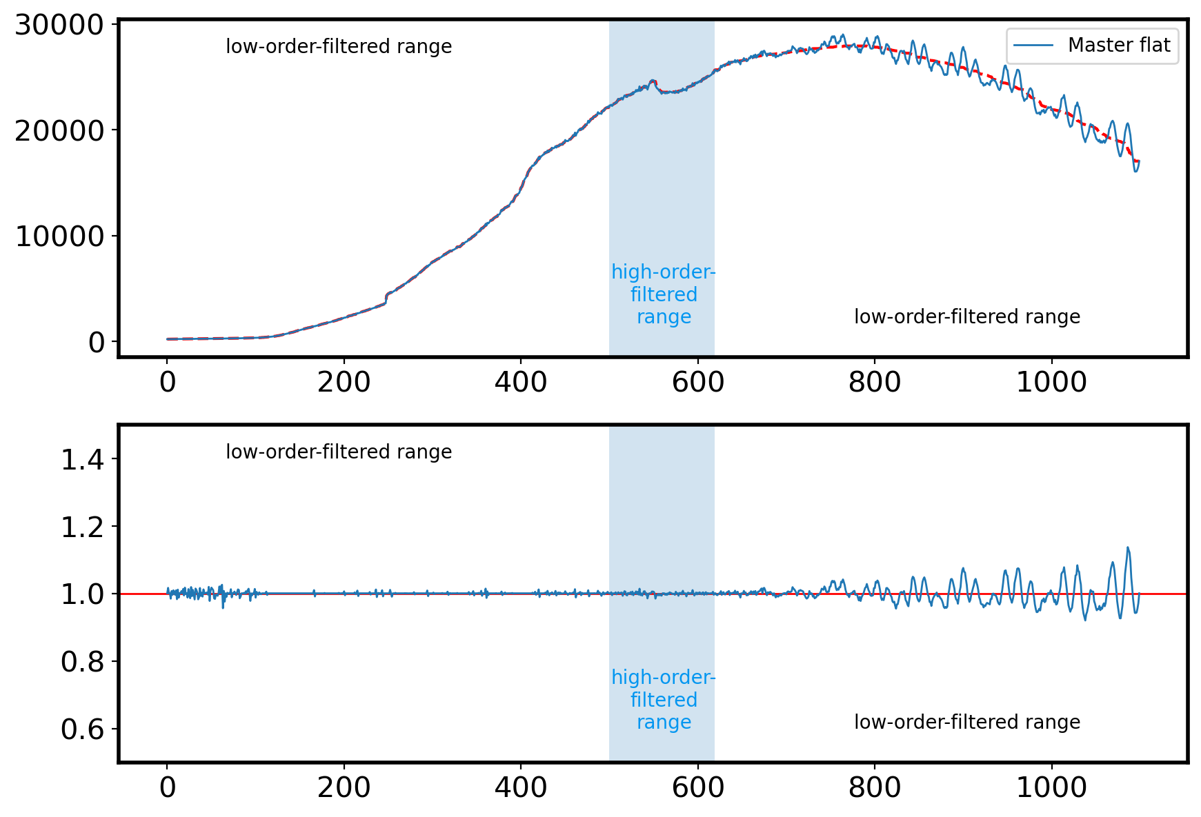
1.4-2 Median combine flat image to make Master Flat#
Note that in our flat frame, both grating-originated wiggles and the lamp-originated bump can be found. Thus we need to account for these effect simultaneously in order to appropriately flat-field our science frame. However, this will be very cumbersome because we need to model our flat spectrum in different regions.
So here we just adopt smoothed flat spectrum with large smoothing scale to normalize the flat (this will effectively play a role of “low-order” fitting), ignoring the bump of the lamp. This will make reduced science spectrum have the bump feature at same location on the dispersion axis.
# Bring Master bias & Dark
biasfile = SUBPATH/'Master_Bias.fits'
Mbias = fits.open(biasfile)[0].data
Mbias = np.array(Mbias).astype('float64')
darkfile = SUBPATH/'Master_Dark_10.0s.fits' # check the exposure time for your flat frames
Mdark = fits.open(darkfile)[0].data
Mdark = np.array(Mdark).astype('float64')
# Make master Flat image
Master_flat = []
for i in range(len(Flatlist)):
hdul = fits.open(Flatlist[i])[0]
header = hdul.header
data = hdul.data
data = np.array(data).astype('float64')
bdata = data - Mbias # bias subtraction
dbdata = bdata - Mdark # dark subtraction
Master_flat.append(dbdata)
MASTER_flat = np.median(Master_flat,axis=0)
header['COMMENT'] = 'Bias_subtraction is done' + datetime.now().strftime('%Y-%m-%d %H:%M:%S (KST)')
header["COMMENT"] = f'{len(Master_dark)} dark images are median combined on '\
+ datetime.now().strftime('%Y-%m-%d %H:%M:%S (KST)')+'with '+' Master_Dark_'+str(exp)+'s.fits'
# normalizing master flat image
flat = np.median(MASTER_flat[115:135,:],axis=0)
fig,ax=plt.subplots(2,1,figsize=(10,7))
ax[0].plot(flat,label='Master flat',lw=1,zorder=20)
# ax[0].set_xlim(200,1500)
ax[0].legend(fontsize=10)
HIGH_WINDOW_LIM = [500, 620] # range limit for low- and high-order median filtering
flat_low1 = flat[:HIGH_WINDOW_LIM[0]]
flat_low2 = flat[HIGH_WINDOW_LIM[1]:]
flat_high = flat[HIGH_WINDOW_LIM[0]:HIGH_WINDOW_LIM[1]]
sflat_low1 = median_filter(flat_low1, 100, mode='nearest') # low-order filtering (left)
sflat_low2 = median_filter(flat_low2, 100, mode='nearest') # low-order filtering (right)
sflat_high = median_filter(flat_high, 10, mode='nearest') # high-order filtering (middle)
sflat = np.hstack([sflat_low1, sflat_high, sflat_low2])
nor_flat = flat/sflat
ax[0].plot(sflat,color='r',ls='--')
ax[1].plot(nor_flat,lw=1,zorder=15)
ax[1].set_ylim(0.5,1.5)
ax[1].axhline(1,color='r',lw=1)
high_window = np.full_like(flat, False)
high_window[HIGH_WINDOW_LIM[0]:HIGH_WINDOW_LIM[1]] = True
for a in ax:
a.fill_between(np.arange(len(flat)),0, 1, where=high_window,
alpha=0.2, transform=a.get_xaxis_transform())
a.text(0.1, 0.9, 'low-order-filtered range', transform=a.transAxes)
a.text(0.51, 0.1, 'high-order-\nfiltered\nrange', transform=a.transAxes,
c='#0296f0', ha='center')
a.text(0.9, 0.1, 'low-order-filtered range', transform=a.transAxes,
ha='right')
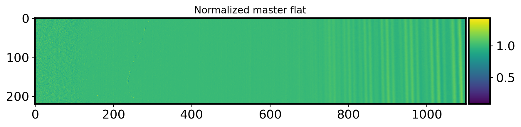
nor_flat2d = []
for i in range(MASTER_flat.shape[0]):
flat = MASTER_flat[i,:]
flat_low1 = flat[:HIGH_WINDOW_LIM[0]]
flat_low2 = flat[HIGH_WINDOW_LIM[1]:]
flat_high = flat[HIGH_WINDOW_LIM[0]:HIGH_WINDOW_LIM[1]]
sflat_low1 = median_filter(flat_low1, 100, mode='nearest') # low-order filtering (left)
sflat_low2 = median_filter(flat_low2, 100, mode='nearest') # low-order filtering (right)
sflat_high = median_filter(flat_high, 10, mode='nearest') # high-order filtering (middle)
sflat = np.hstack([sflat_low1, sflat_high, sflat_low2])
nor_flat2d.append(flat / sflat)
nor_flat2d = np.array(nor_flat2d)
header['COMMENT'] = 'Normalized' + datetime.now().strftime('%Y-%m-%d %H:%M:%S (KST)')
SAVE_flat = SUBPATH/'Master_Flat.fits'
fits.writeto(SAVE_flat, nor_flat2d, header=header, overwrite=True)
fig,ax = plt.subplots(1,1,figsize=(10,5))
im=ax.imshow(nor_flat2d)
divider = make_axes_locatable(ax)
cax = divider.append_axes("right",size='5%',pad=0.05)
plt.colorbar(im,cax=cax)
ax.set_title('Normalized master flat')
Text(0.5, 1.0, 'Normalized master flat')
1.5 Master Calibration image#
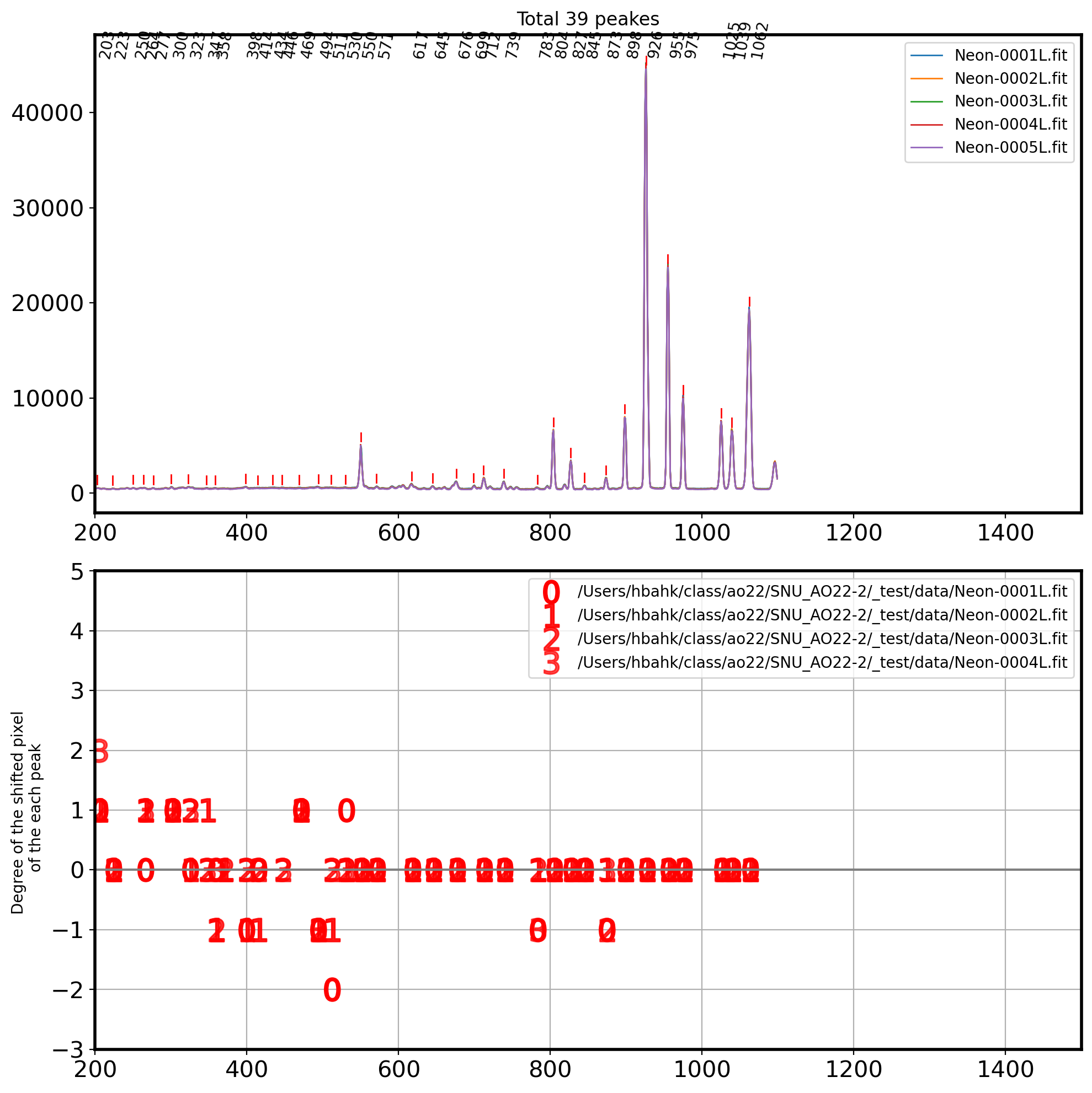
Check wavelength Calibration image shift#
I will check the wavelength calibration image shift with the same manner done for flat image.
# Bring Master bias & Dark
biasfile = os.path.join(SUBPATH,'Master_Bias.fits')
Mbias = fits.open(biasfile)[0].data
Mbias = np.array(Mbias).astype('float64')
darkfile = os.path.join(SUBPATH,'Master_Dark_60.0s.fits')
Mdark = fits.open(darkfile)[0].data
Mdark = np.array(Mdark).astype('float64')
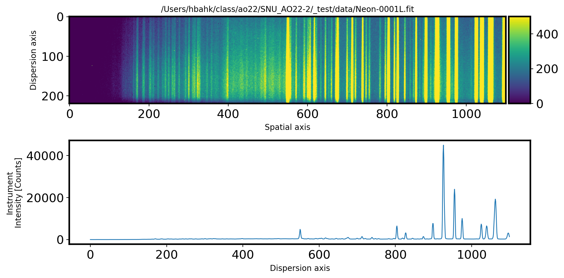
# Plot the Comparison image
fig, ax = plt.subplots(2, 1, figsize=(10, 5))
hdul = fits.open(Complist[0])[0]
data = hdul.data
data = np.array(data).astype('float64')
data = data - Mbias - Mdark
im = ax[0].imshow(data, vmin=0, vmax=500)
divider = make_axes_locatable(ax[0])
cax = divider.append_axes("right", size='5%', pad=0.05)
plt.colorbar(im,cax=cax)
ax[0].set_title(Complist[0], fontsize=10)
ax[0].set_xlabel('Spatial axis')
ax[0].set_ylabel('Dispersion axis')
# Cut the spectrum along the dispersion direction
ComSpec = np.median(data[115:135,:], axis=0)
ax[1].plot(ComSpec, lw=1)
ax[1].set_xlabel('Dispersion axis')
ax[1].set_ylabel('Instrument\nIntensity [Counts]')
plt.tight_layout()
# Find the local peak for each image

fig,ax = plt.subplots(2,1,figsize=(10,10))
Coor_shift = []
for i in range(len(Complist)):
    hdul = fits.open(Complist[i])[0]
    data = hdul.data
    data = np.array(data).astype('float64')
    neon = np.median(data[115:135,:],axis=0)

    ax[0].plot(neon,label=Complist[i].name,lw=1)
    ax[0].set_xlim(200,1500)
    ax[0].legend(fontsize=10)


    x = np.arange(0,len(neon))
    # peak finding
    coordinates = peak_local_max(neon, min_distance=10,
                                 threshold_abs=max(neon)*0.01)

    Coor_shift.append(coordinates) # to compare peak locations frame by frame

ax[0].set_title('Total {0} peakes'.format(int(len(coordinates))))

for i in coordinates:
    ax[0].annotate(i[0],(i,max(neon)+ max(neon)*0.03),
                  fontsize=10,rotation=80)
    ax[0].plot([i,i],
            [neon[i] + max(neon)*0.01, neon[i] + max(neon)*0.03],
            color='r',lw=1)

reference_coor = sorted(Coor_shift[0])

for i in range(len(Coor_shift)-1):
    coor_i = Coor_shift[i+1]
    x_shift = []
    y_shift = []
    for k in range(len(reference_coor)):
        for t in range(len(coor_i)):
            if abs(reference_coor[k]-coor_i[t]) <5 :
                y_shift.append(reference_coor[k]-coor_i[t])
                x_shift.append(reference_coor[k])
    ax[1].plot(x_shift,y_shift,ls='',marker=f'${int(i)}$',
               markersize=15,color='r',alpha=1-i*0.1, label=Complist[i])
ax[1].set_xlim(200, 1500)
ax[1].set_ylim(-3, 5)
ax[1].set_ylabel('Degree of the shifted pixel \n of the each peak')
ax[1].axhline(0,color='gray')
ax[1].grid()
ax[1].legend()

plt.tight_layout()
Median combine Comparison Lamp image#
Master_Comp = []
for i in range(len(Complist)):
    hdul = fits.open(Complist[i])[0]
    header = hdul.header
    data = hdul.data
    data = data - Mbias - Mdark

    Master_Comp.append(data)

MASTER_Comp = np.median(Master_Comp,axis=0)
SAVE_comp = os.path.join(SUBPATH,'Master_Neon.fits')
fits.writeto(SAVE_comp,MASTER_Comp,header = header,overwrite=True)
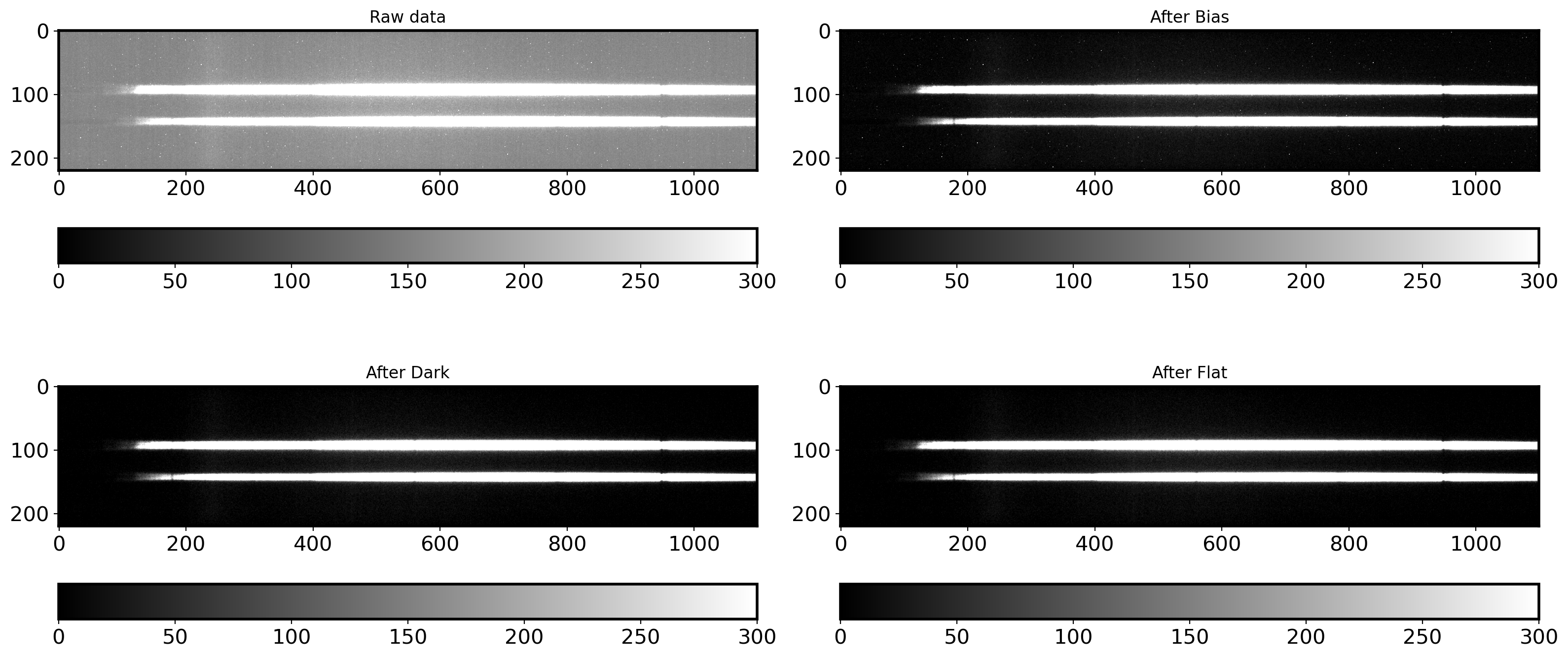
1.6 Bias subtraction & Dark subtraction (Pre-Processing)#
# Bring the sample image
raw_data = SUBPATH/'61Cygni-0001.fit'
objhdul = fits.open(raw_data)
raw_data = objhdul[0].data

# Bring Master Bias
biasfile = SUBPATH/'Master_Bias.fits'
Mbias = fits.open(biasfile)[0].data
Mbias = np.array(Mbias).astype('float64')

# Bring Master Dark
darkfile = SUBPATH/'Master_Dark_2.0s.fits'
Mdark = fits.open(darkfile)[0].data
Mdark = np.array(Mdark).astype('float64')

# Bring Master Flat
flatfile = SUBPATH/'Master_Flat.fits'
Mflat = fits.open(flatfile)[0].data
Mflat = np.array(Mflat).astype('float64')


# Bias subtracting
bobjdata = raw_data - Mbias

# Dark_subtracting
dbobjdata = bobjdata - Mdark

# Flat fielding
fdbobjdata = dbobjdata / Mflat


fig,ax = plt.subplots(2,2,figsize=(16,8))
ax1 = ax[0,0].imshow(raw_data,vmin=0,vmax=300,cmap='gray')
fig.colorbar(ax1, ax=ax[0,0],orientation = 'horizontal')
ax[0,0].set_title('Raw data')


ax2 = ax[0,1].imshow(bobjdata,vmin=0,vmax=300,cmap='gray')
fig.colorbar(ax2, ax=ax[0,1],orientation = 'horizontal')
ax[0,1].set_title('After Bias')

ax3 = ax[1,0].imshow(dbobjdata,vmin=0,vmax=300,cmap='gray')
fig.colorbar(ax3, ax=ax[1,0],orientation = 'horizontal')
ax[1,0].set_title('After Dark')

ax4 = ax[1,1].imshow(fdbobjdata,vmin=0,vmax=300,cmap='gray')
fig.colorbar(ax3, ax=ax[1,1],orientation = 'horizontal')
ax[1,1].set_title('After Flat')

plt.tight_layout()
# Do it for all object image

OBJ = np.concatenate([Objectlist,Standlist])
for i in range(len(OBJ)):
    # Bring the sample image
    objhdul = fits.open(OBJ[i])
    raw_data = objhdul[0].data
    header = objhdul[0].header

    # Bring Master Bias
    biasfile = SUBPATH/'Master_Bias.fits'
    Mbias = fits.open(biasfile)[0].data
    Mbias = np.array(Mbias).astype('float64')

    # Bring Master Dark
    EXPTIME = objhdul[0].header['EXPTIME']
    darkfile = SUBPATH/f'Master_Dark_{EXPTIME:.1f}s.fits'
    Mdark = fits.open(darkfile)[0].data
    Mdark = np.array(Mdark).astype('float64')

    # Bring Master Dark
    flatfile = SUBPATH/f'Master_Flat.fits'
    Mflat = fits.open(flatfile)[0].data
    Mflat = np.array(Mflat).astype('float64')

    # Bias subtracting
    bobjdata = raw_data - Mbias

    # Dark subtracting
    dbobjdata = bobjdata - Mdark

    # Flat fielding
    fdbobjdata = dbobjdata / Mflat

    # Add header comment
    header['COMMENT'] = 'Bias_subtraction is done' + datetime.now().strftime('%Y-%m-%d %H:%M:%S (KST)')
    header["COMMENT"]='{0} dark images are median combined on '.format(len(Master_dark))\
    + datetime.now().strftime('%Y-%m-%d %H:%M:%S (KST)')+ 'with '+' Master_Dark_'+str(exp)+'s.fits'

    # Save the image
    SAVE_name = SUBPATH/('p'+ OBJ[i].name+'s')
    fits.writeto(SAVE_name, fdbobjdata, header=header, overwrite=True)
    print(SAVE_name,' is made!')

# comparison lamp frame
Master_comparison = SUBPATH/'Master_Neon.fits'
hdul = fits.open(Master_comparison)[0]
data = hdul.data

fits.writeto(SUBPATH/'pMaster_Neon.fits', data, header=hdul.header, overwrite=True)
/Users/hbahk/class/ao22/SNU_AO22-2/_test/data/p61Cygni-0001.fits  is made!
/Users/hbahk/class/ao22/SNU_AO22-2/_test/data/p61Cygni-0002.fits  is made!
/Users/hbahk/class/ao22/SNU_AO22-2/_test/data/p61Cygni-0003.fits  is made!
/Users/hbahk/class/ao22/SNU_AO22-2/_test/data/p61Cygni-0004.fits  is made!
/Users/hbahk/class/ao22/SNU_AO22-2/_test/data/p61Cygni-0005.fits  is made!
/Users/hbahk/class/ao22/SNU_AO22-2/_test/data/pHR153-0001.fits  is made!
/Users/hbahk/class/ao22/SNU_AO22-2/_test/data/pHR153-0002.fits  is made!
/Users/hbahk/class/ao22/SNU_AO22-2/_test/data/pHR153-0003.fits  is made!
/Users/hbahk/class/ao22/SNU_AO22-2/_test/data/pHR153-0004.fits  is made!
/Users/hbahk/class/ao22/SNU_AO22-2/_test/data/pHR153-0005.fits  is made!
2. Spectroscopic data reduction#
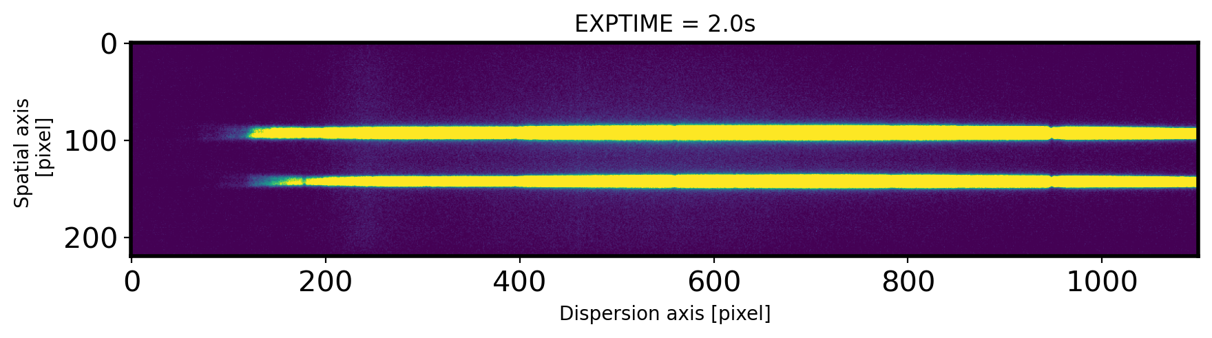
2-1. Extract the Spectrum#
Identification of Object’s peak & Set the area of background#
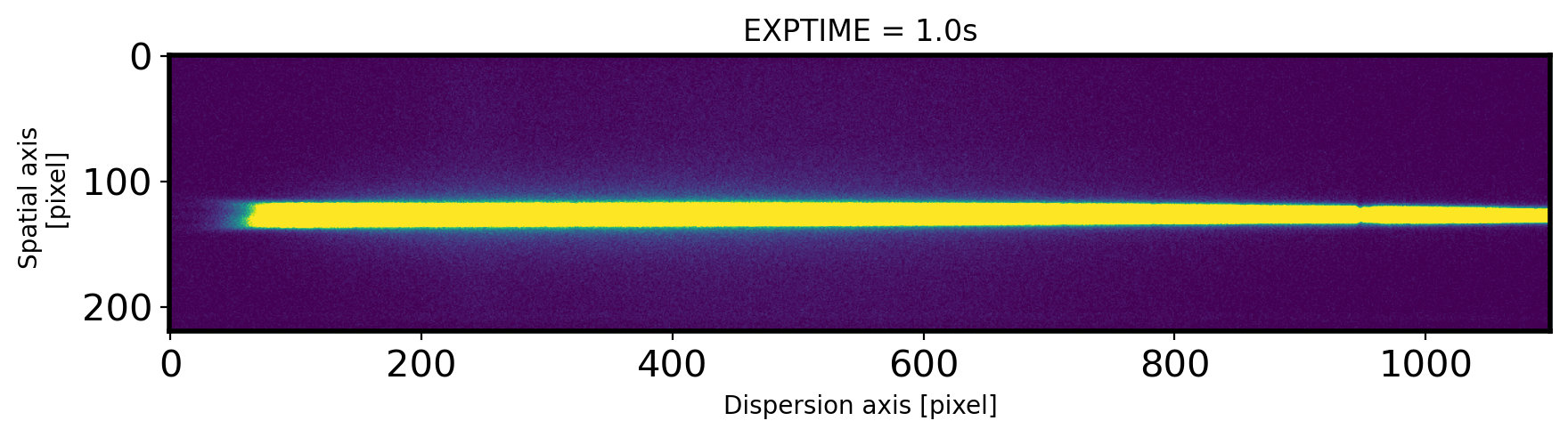
# Bring the sample image

OBJECTNAME = SUBPATH/'p61Cygni-0001.fits'
hdul = fits.open(OBJECTNAME)[0]
obj = hdul.data
header = hdul.header
EXPTIME = header['EXPTIME']
fig,ax = plt.subplots(1,1,figsize=(10,15))
ax.imshow(obj,vmin=0,vmax=300)
ax.set_title('EXPTIME = {0}s'.format(EXPTIME))
ax.set_xlabel('Dispersion axis [pixel]')
ax.set_ylabel('Spatial axis \n [pixel]')
Text(0, 0.5, 'Spatial axis \n [pixel]')
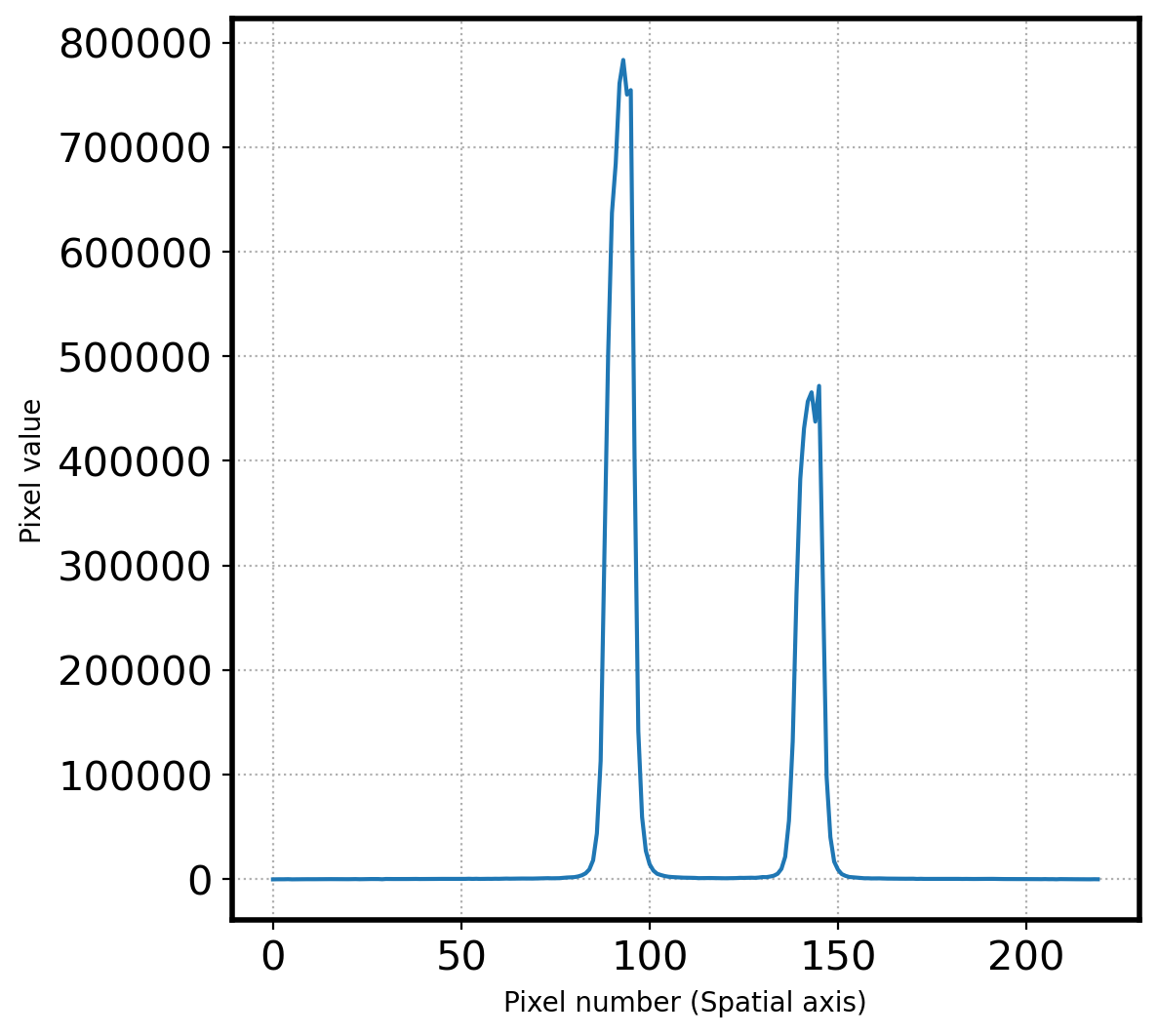
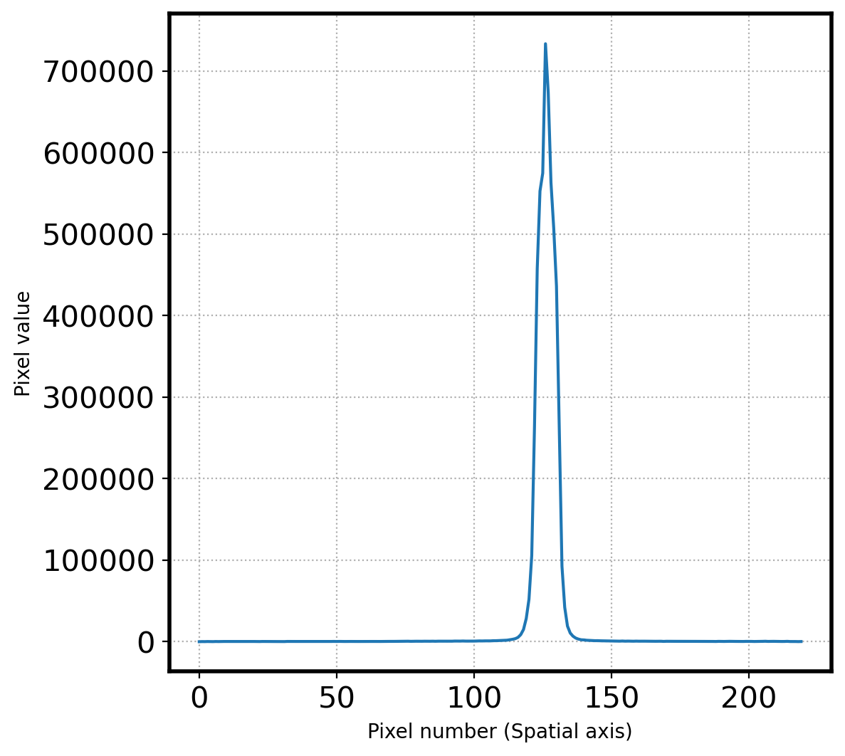
# Let's find the peak along the spatial axis

# Plot the spectrum along the spatial direction
lower_cut = 700
upper_cut = 750
apall_1 = np.sum(obj[:,lower_cut:upper_cut],axis=1)

fig, ax = plt.subplots(1,1,figsize=(6,6))
ax.plot(apall_1)
ax.set_xlabel('Pixel number (Spatial axis)')
ax.set_ylabel('Pixel value')
ax.grid(ls=':')

# Find the peak

peak_pix = peak_local_max(apall_1, num_peaks=10,
                          min_distance=30,
                          threshold_abs=np.median(apall_1))
peak_pix = np.array(peak_pix[:,0])
print(peak_pix)

fig,ax = plt.subplots(1,1,figsize=(6,6))
x = np.arange(0, len(apall_1))
ax.plot(x, apall_1)
ax.set_xlabel('Spatial axis')

peak_value = []
for i in peak_pix:
    ax.plot((i, i),
            (apall_1[i]+0.01*max(apall_1),apall_1[i]+0.1*max(apall_1)),
            color='r', ls='-', lw=1)
    ax.annotate(i, (i, apall_1[i]+0.1*max(apall_1)),
            fontsize='small', rotation=45)
    peak_value.append(apall_1[i])
    print(i)

peak_pix = np.sort(peak_pix)

ax.grid(ls=':')
ax.set_xlabel('Pixel number (Spatial axis)')
ax.set_ylabel('Pixel value')

plt.show()

print(f'Pixel coordinatate in spatial direction = {peak_pix}')
[145  93]
145
93
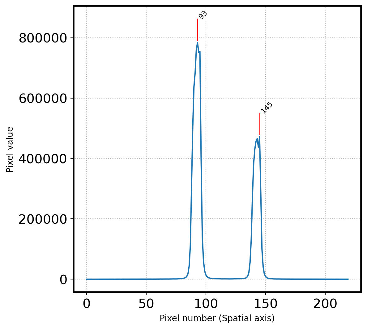
Pixel coordinatate in spatial direction = [ 93 145]
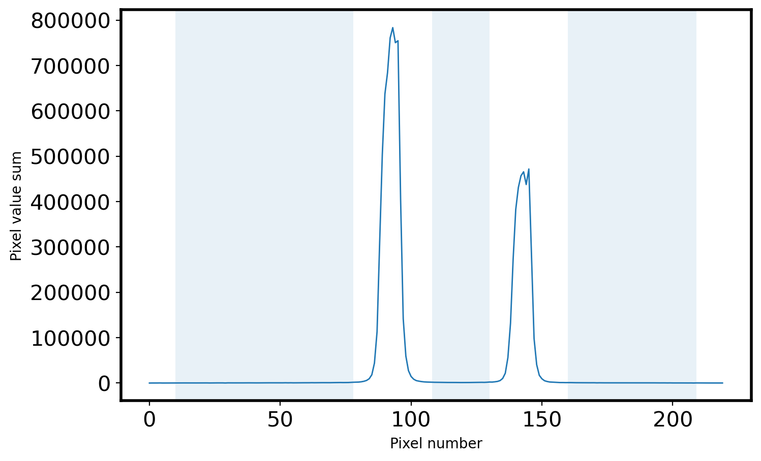
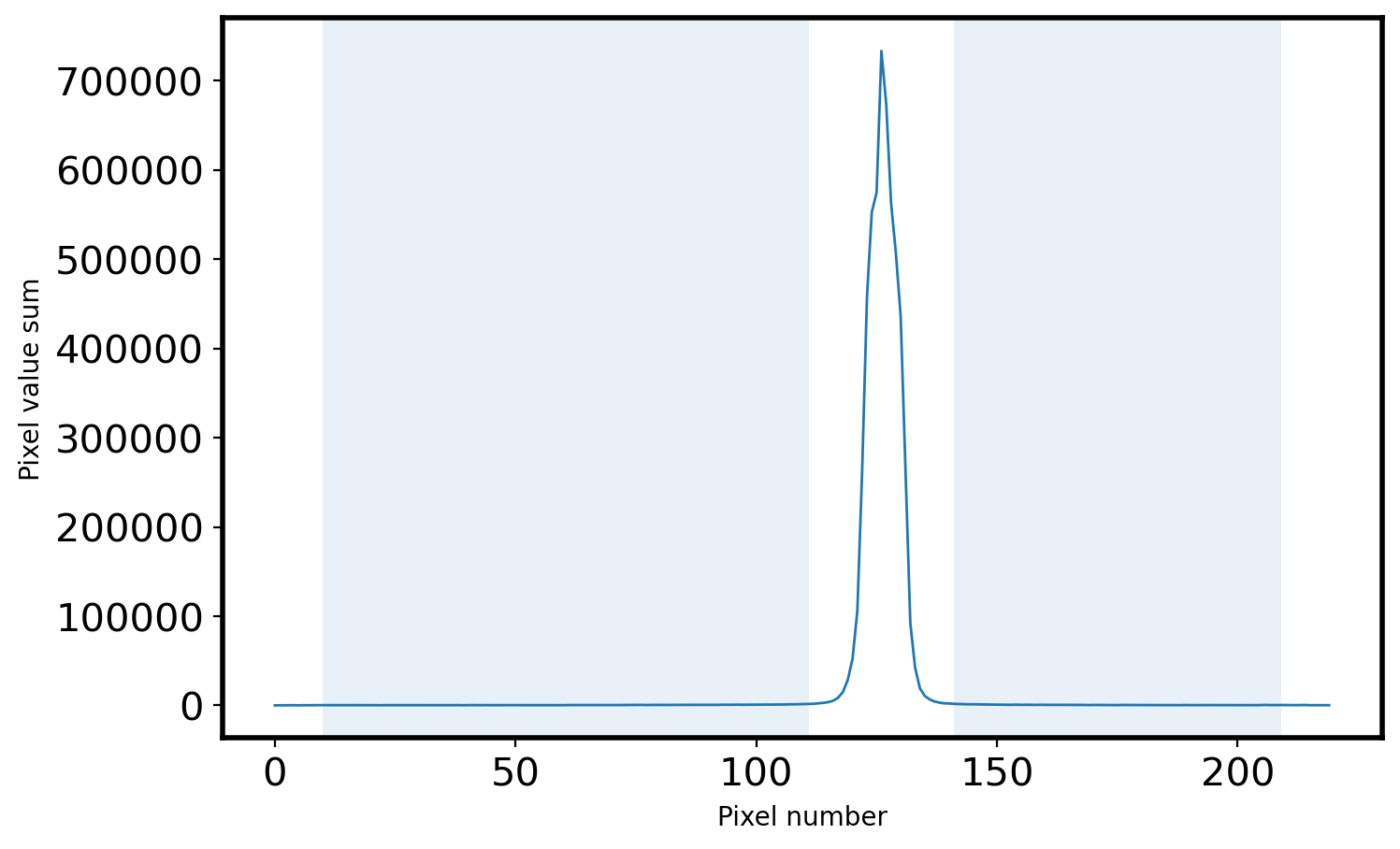
# Select the sky area
peak = peak_pix[0] # center
print('Peak pixel is {0} pix'.format(peak_pix[0]))

SKYLIMIT = 15 # pixel limit around the peak
RLIMIT = 10 # pixel limit from the rightmost area
LLIMIT = 10 # pixel limit from the leftmost area

mask_sky = np.full_like(x, True, dtype=bool)
for p in peak_pix:
    mask_sky[(x > p-SKYLIMIT) & (x < p+SKYLIMIT)] = False
mask_sky[:LLIMIT] = False
mask_sky[-RLIMIT:] = False

x_sky = x[mask_sky]
sky_val = apall_1[mask_sky]

# Plot the sky area
fig = plt.figure(figsize=(8, 5))
ax = fig.add_subplot(111)
ax.plot(x, apall_1, lw=1)
ax.fill_between(x, 0, 1, where=mask_sky, alpha=0.1, transform=ax.get_xaxis_transform())

ax.set_xlabel('Pixel number')
ax.set_ylabel('Pixel value sum')
Peak pixel is 93 pix
Text(0, 0.5, 'Pixel value sum')
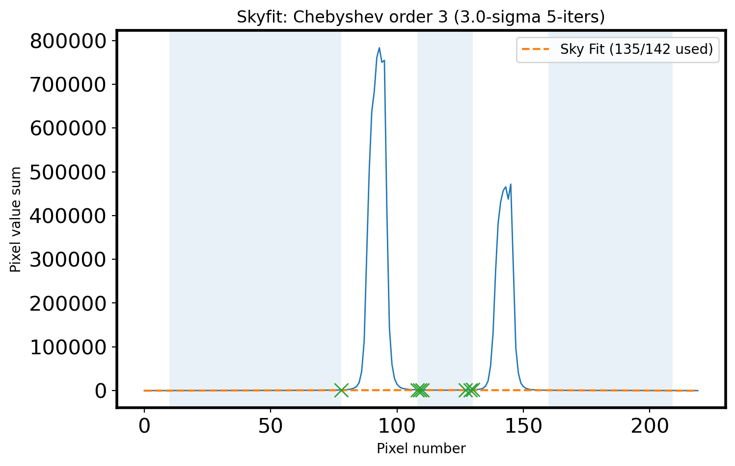
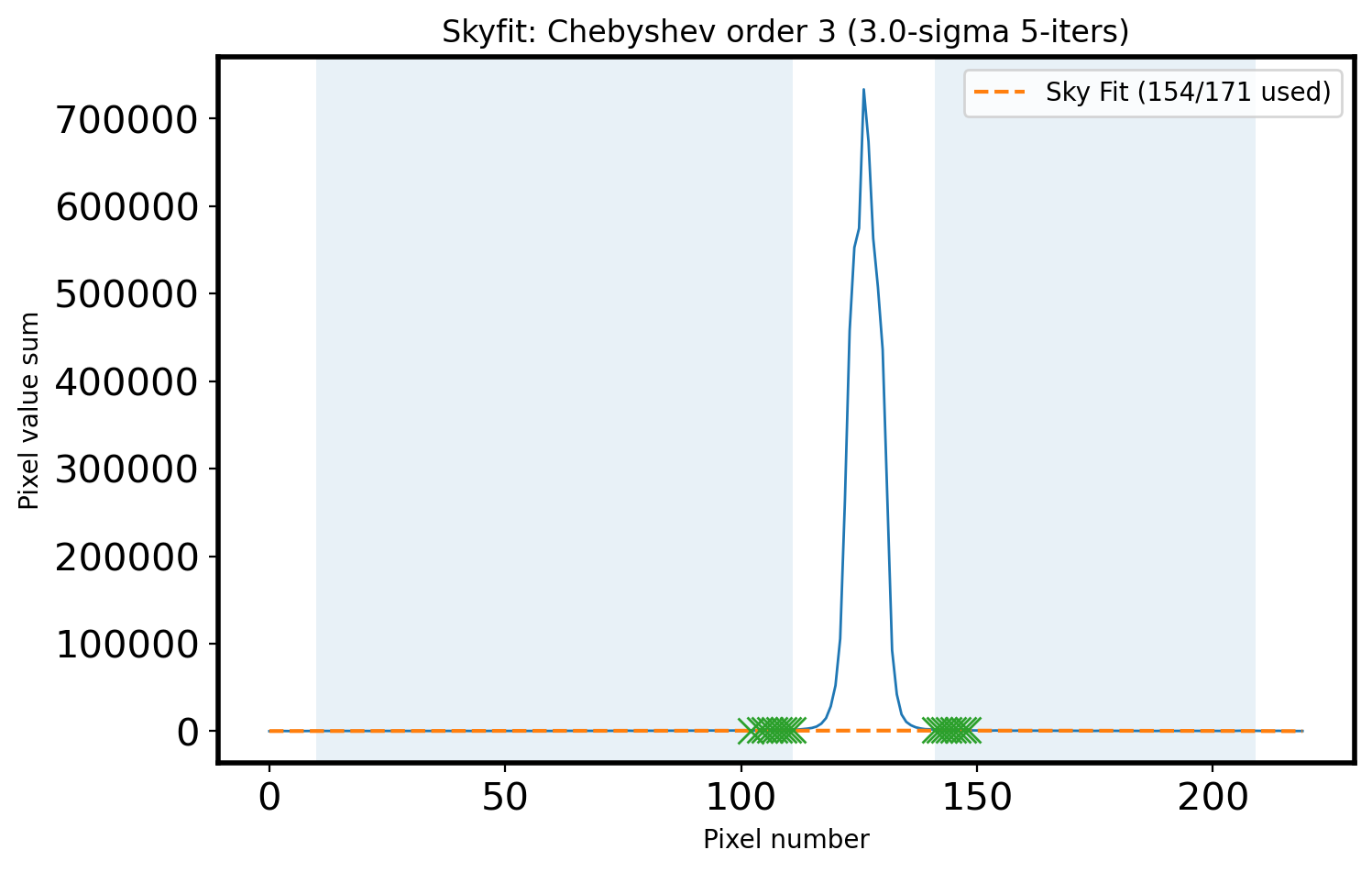
# Sigma clipping
Sigma = 3
clip_mask = sigma_clip(sky_val,
                       sigma=Sigma,
                       maxiters= 5).mask

# Fit the sky
ORDER_APSKY = 3
coeff_apsky, fitfull = chebfit(x_sky[~clip_mask],
                               sky_val[~clip_mask],
                               deg=ORDER_APSKY,
                               full=True)
sky_fit = chebval(x, coeff_apsky)

# Calculate the RMS of Fit
residual = fitfull[0][0]
fitRMS = np.sqrt(residual/len(x_sky[~clip_mask]))


n_sky = len(x_sky)
n_rej = np.count_nonzero(clip_mask)

# Plot the sky area & fitted sky
fig,ax = plt.subplots(1,1,figsize=(8, 5))

ax.plot(x, apall_1, lw=1)
ax.plot(x, sky_fit, ls='--',
        label='Sky Fit ({:d}/{:d} used)'.format(n_sky - n_rej, n_sky))
ax.plot(x_sky[clip_mask], sky_val[clip_mask], marker='x', ls='', ms=10)
ax.fill_between(x, 0, 1, where=mask_sky, alpha=0.1, transform=ax.get_xaxis_transform())


title_str = r'Skyfit: {:s} order {:d} ({:.1f}-sigma {:d}-iters)'
ax.set_xlabel('Pixel number')
ax.set_ylabel('Pixel value sum')
ax.legend()
ax.set_title(title_str.format('Chebyshev', ORDER_APSKY,
                              Sigma, 5))
Text(0.5, 1.0, 'Skyfit: Chebyshev order 3 (3.0-sigma 5-iters)')
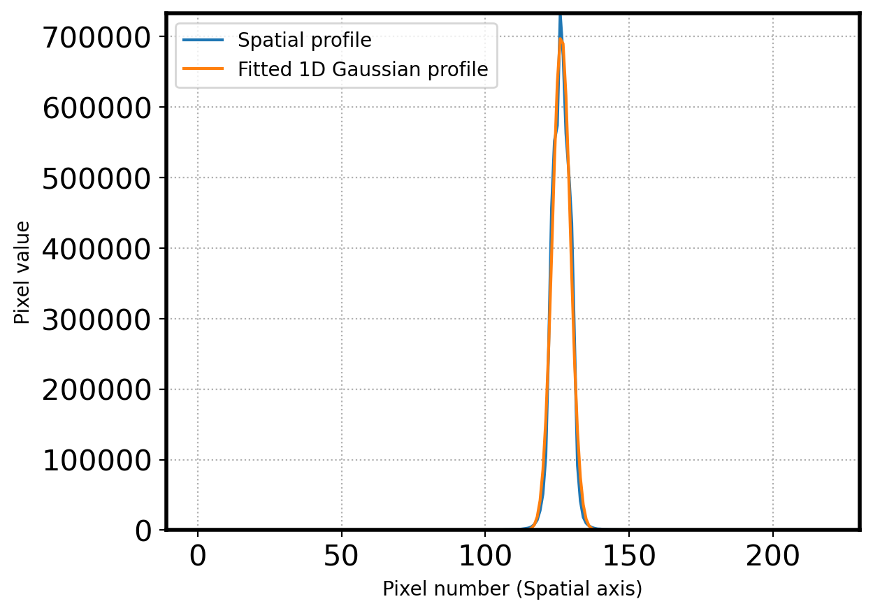
# Finding the peak center by fitting the gaussian 1D function again

sub_apall_1 = apall_1 - sky_fit # profile - sky

# OUTPIX = 50 # number of pixels to rule out outermost area in spacial direction
# xx = x[OUTPIX:-OUTPIX]
# yy = sub_apall_1[OUTPIX:-OUTPIX]

xx = x[peak-SKYLIMIT:peak+SKYLIMIT]
yy = sub_apall_1[peak-SKYLIMIT:peak+SKYLIMIT]

# gaussian modeling
g_init = Gaussian1D(amplitude=sub_apall_1[peak],
                    mean=peak,
                    stddev=15*gaussian_fwhm_to_sigma)

fitter = LevMarLSQFitter()
fitted = fitter(g_init, xx, yy)

params = [fitted.amplitude.value, fitted.mean.value, fitted.stddev.value]

fig = plt.figure()
ax = fig.add_subplot(111)
x = np.arange(0, len(apall_1))
ax.plot(x, sub_apall_1, label='Spatial profile')

g = Gaussian1D(*params)

ax.plot(x, g(x), label='Fitted 1D Gaussian profile')
ax.grid(ls=':')
ax.set_xlabel('Pixel number (Spatial axis)')
ax.set_ylabel('Pixel value')
ax.set_ylim(0, sub_apall_1[peak])
ax.legend(loc=2,fontsize=10)
plt.show()

center_pix = params[1]
print('center pixel:', center_pix)
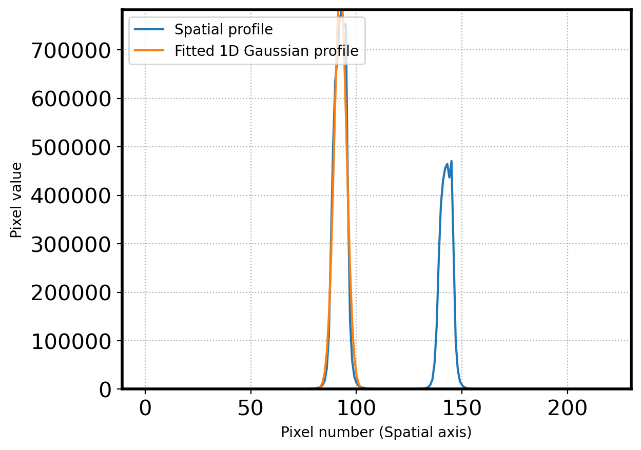
center pixel: 92.4245791504611
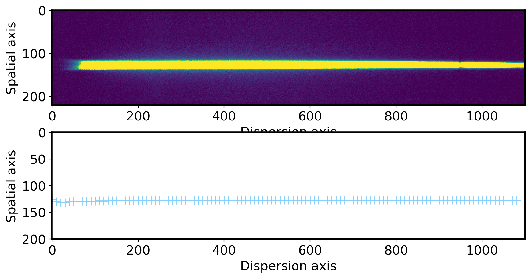
# Trace the aperture (peak) along the wavelength.
# Repeat the above process for all wavelength bands.
# This process is called "aperture tracing".
aptrace = []
aptrace_fwhm = []
STEP_AP = 10
N_AP = len(obj[0])//STEP_AP
FWHM_AP = 10
peak = center_pix
for i in range(N_AP - 1):
    lower_cut, upper_cut = i*STEP_AP, (i+1)*STEP_AP
    apall_i = np.sum(obj[:, lower_cut:upper_cut], axis=1)
    sky_val = apall_i[mask_sky]
    clip_mask = sigma_clip(sky_val,
                           sigma=3,
                           maxiters=5).mask
    coeff, fitfull = chebfit(x_sky[~clip_mask],
                             sky_val[~clip_mask],
                             deg=ORDER_APSKY,
                             full=True)
    apall_i -= chebval(x,coeff)  # Object profile - the fitted sky

    search_min = int(peak - 3*FWHM_AP)
    search_max = int(peak + 3*FWHM_AP)
    cropped = apall_i[search_min:search_max]
    x_cropped = np.arange(len(cropped))

    peak_pix_trace = peak_local_max(cropped,
                              min_distance=FWHM_AP,
                              num_peaks=1)
    peak_pix_trace = np.array(peak_pix_trace[:,0])

    if len(peak_pix_trace) == 0: # return NaN (Not a Number) if there is no peak found.
        aptrace.append(np.nan)
        aptrace_fwhm.append(0)
    else:
        peak_pix_trace = np.sort(peak_pix_trace)
        peak_trace = peak_pix_trace[0]
        g_init = Gaussian1D(amplitude=cropped[peak_trace], # Gaussian fitting to find centers
                            mean=peak_trace,
                            stddev=FWHM_AP*gaussian_fwhm_to_sigma,
                            bounds={'amplitude':(0, 2*cropped[peak_trace]) ,
                                    'mean':(peak_trace-3*FWHM_AP, peak_trace+3*FWHM_AP),
                                    'stddev':(0.00001, FWHM_AP*gaussian_fwhm_to_sigma)})
        fitted = fitter(g_init, x_cropped, cropped)
        center_pix_new = fitted.mean.value + search_min
        aptrace_fwhm.append(fitted.fwhm)
        aptrace.append(center_pix_new)

aptrace = np.array(aptrace)
aptrace_fwhm = np.array(aptrace_fwhm)
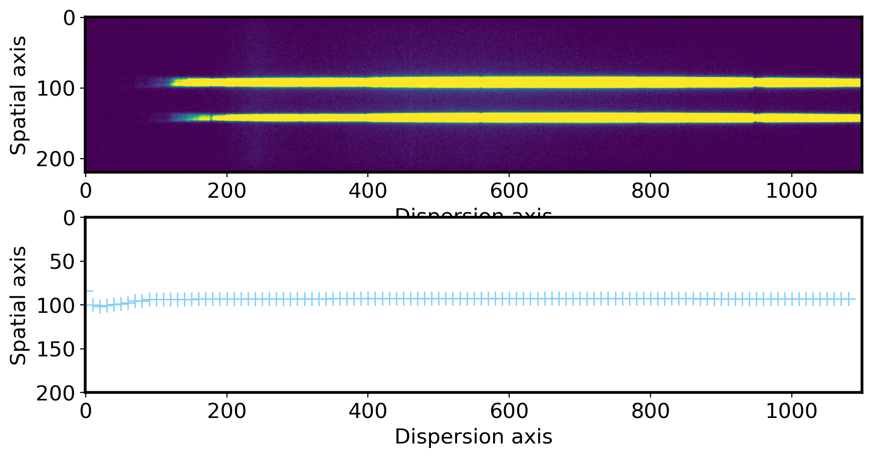
# Plot the center of profile peak
fig,ax = plt.subplots(2,1,figsize=(10,5))
ax[0].imshow(obj,vmin=0,vmax=300)
ax[0].set_xlabel('Dispersion axis',fontsize=15)
ax[0].set_ylabel('Spatial axis',fontsize=15)
xlim = ax[0].get_xlim()

ax[1].plot(np.arange(len(aptrace))*10, aptrace,ls='', marker='+', ms=10,color='lightskyblue')
ax[1].set_xlim(xlim)
ax[1].set_ylim(200,0) # you can see the jiggly-wiggly shape when you zoom in
ax[1].set_xlabel('Dispersion axis',fontsize=15)
ax[1].set_ylabel('Spatial axis',fontsize=15)
Text(0, 0.5, 'Spatial axis')
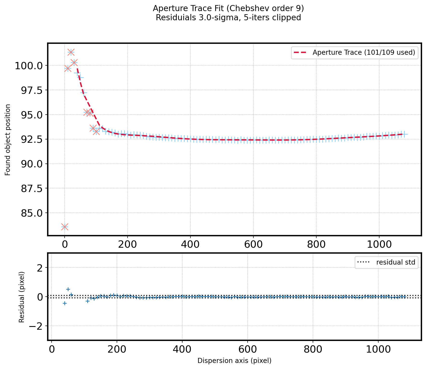
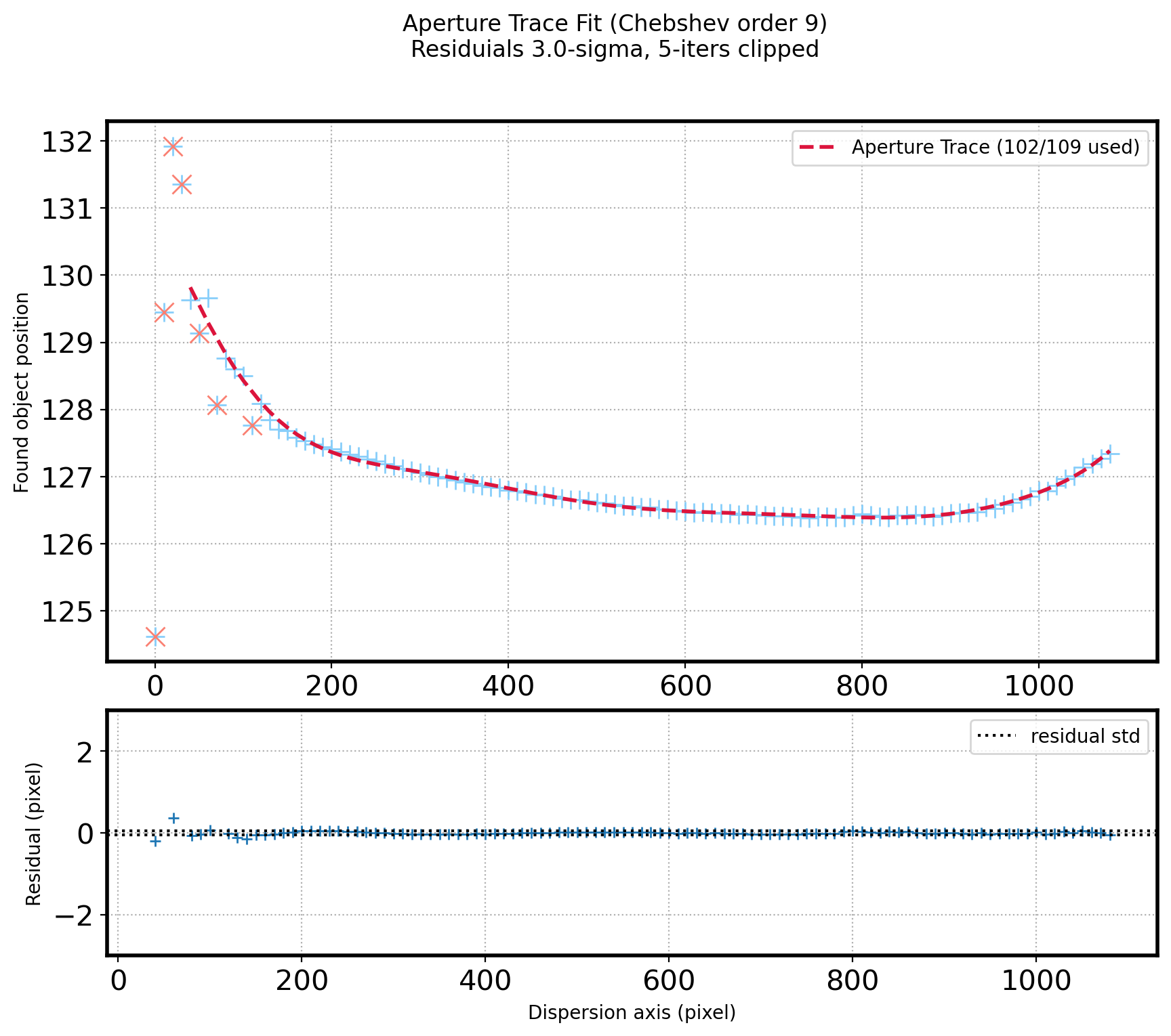
# Fitting the peak with Chebyshev function

ORDER_APTRACE = 9
SIGMA_APTRACE = 3
ITERS_APTRACE = 5 # when sigma clipping

# Fitting the line
x_aptrace = np.arange(N_AP-1) * STEP_AP
coeff_aptrace = chebfit(x_aptrace, aptrace, deg=ORDER_APTRACE)

# Sigma clipping
resid_mask = sigma_clip(aptrace - chebval(x_aptrace, coeff_aptrace),
                        sigma=SIGMA_APTRACE, maxiters=ITERS_APTRACE).mask

# Fitting the peak again after sigma clipping
x_aptrace_fin = x_aptrace[~resid_mask]
aptrace_fin = aptrace[~resid_mask]
coeff_aptrace_fin = chebfit(x_aptrace_fin, aptrace_fin, deg=ORDER_APTRACE)

fit_aptrace_fin   = chebval(x_aptrace_fin, coeff_aptrace_fin)
resid_aptrace_fin = aptrace_fin - fit_aptrace_fin
del_aptrace = ~np.in1d(x_aptrace, x_aptrace_fin) # deleted points #x_aptrace에서 x_aptrace_fin이 없으면 True
'''
test = np.array([0, 1, 2, 5, 0])
states = [0, 2]
mask = np.in1d(test, states)
mask
array([ True, False,  True, False,  True])
'''


# Plot the Fitted line & residual
fig = plt.figure(figsize=(10,8))
gs = gridspec.GridSpec(3, 1)
ax1 = plt.subplot(gs[0:2])
ax2 = plt.subplot(gs[2])

ax1.plot(x_aptrace, aptrace, ls='', marker='+', ms=10,color='lightskyblue')
ax1.plot(x_aptrace_fin, fit_aptrace_fin, ls='--',color='crimson',zorder=10,lw=2,
         label="Aperture Trace ({:d}/{:d} used)".format(len(aptrace_fin), N_AP-1))
ax1.plot(x_aptrace[del_aptrace], aptrace[del_aptrace], ls='', marker='x',color='salmon', ms=10)
ax1.set_ylabel('Found object position')
ax1.grid(ls=':')
ax1.legend()


ax2.plot(x_aptrace_fin, resid_aptrace_fin, ls='', marker='+')
ax2.axhline(+np.std(resid_aptrace_fin, ddof=1), ls=':', color='k')
ax2.axhline(-np.std(resid_aptrace_fin, ddof=1), ls=':', color='k',
            label='residual std')


ax2.set_ylabel('Residual (pixel)')
ax2.set_xlabel('Dispersion axis (pixel)')

ax2.grid(ls=':')
ax2.set_ylim(-3, 3)
ax2.legend()

#Set plot title
title_str = ('Aperture Trace Fit ({:s} order {:d})\n'
            + 'Residuials {:.1f}-sigma, {:d}-iters clipped')
plt.suptitle(title_str.format('Chebshev', ORDER_APTRACE,
                              SIGMA_APTRACE, ITERS_APTRACE))
plt.show()
# Aperture sum

apsum_sigma_lower = 3 # [Sigma]
apsum_sigma_upper = 3
ap_fwhm = np.median(aptrace_fwhm[~resid_mask]) # [pix]
ap_sigma = ap_fwhm * gaussian_fwhm_to_sigma # [pixel/sigma]
x_ap = np.arange(len(obj[0])) # pixel along the dispersion axis
y_ap = chebval(x_ap, coeff_aptrace_fin) # center of peak for each line

# Extract the spectrum along the dispersion axis
ap_summed  = []
ap_sig = []

for i in range(len(obj[0])):
    cut_i = obj[:,i] # Cut spatial direction
    peak_i = y_ap[i]
    offset_i = peak_i - peak

    mask_sky_i = np.full_like(x, True, dtype=bool)
    for p in peak_pix:
        mask_sky_i[(x > p+offset_i-SKYLIMIT) & (x < p+offset_i+SKYLIMIT)] = False
    mask_sky_i[:LLIMIT] = False
    mask_sky_i[-RLIMIT:] = False

    # aperture size = apsum_sigma_lower * ap_sigma
    x_obj_lower = int(np.around(peak_i - apsum_sigma_lower * ap_sigma))
    x_obj_upper = int(np.around(peak_i + apsum_sigma_upper * ap_sigma))
    x_obj = np.arange(x_obj_lower, x_obj_upper)
    obj_i = cut_i[x_obj_lower:x_obj_upper]

    # Fitting Sky value
    x_sky = x[mask_sky_i]
    sky_val = cut_i[mask_sky_i]
    clip_mask = sigma_clip(sky_val, sigma=Sigma,
                           maxiters=5).mask
    coeff = chebfit(x_sky[~clip_mask],
                    sky_val[~clip_mask],
                    deg=ORDER_APSKY)

    # Subtract the sky
    sub_obj_i = obj_i - chebval(x_obj, coeff) # obj - lsky  subtraction


    # Calculate error
    sig_i = RN **2 + sub_obj_i + chebval(x_obj,coeff)
    # RN**2 + flux_i + sky value

    ap_summed.append(np.sum(sub_obj_i))
    ap_sig.append(np.sqrt(np.sum(sig_i)))

ap_summed = np.array(ap_summed) / EXPTIME
ap_std = np.array(ap_sig) / EXPTIME
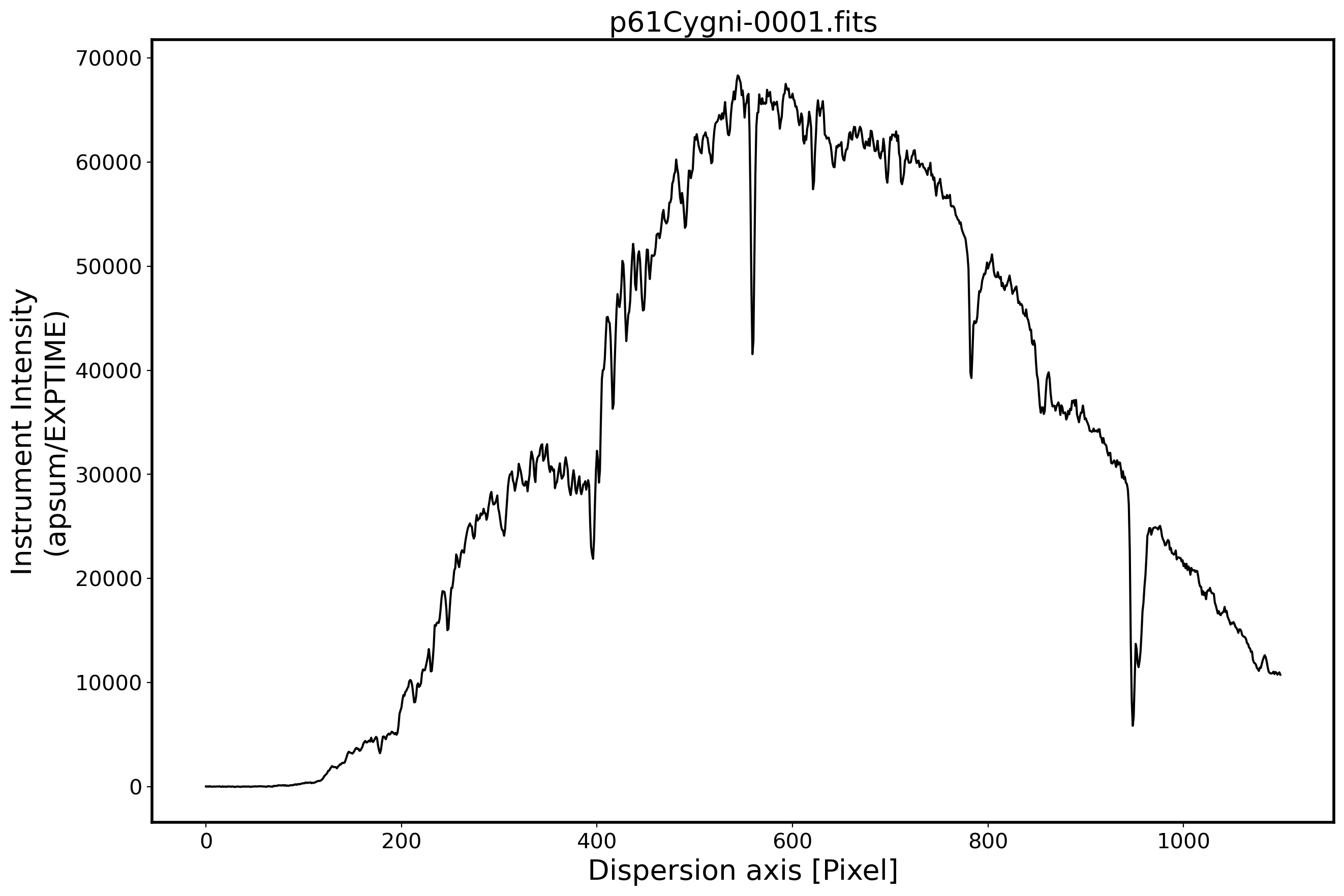
# Plot the spectrum

x_pix = np.arange(len(obj[0]))

fig,ax = plt.subplots(1,1,figsize=(15,10))
ax.plot(x_pix,ap_summed,color='k',alpha=1)


FILENAME = OBJECTNAME.name
ax.set_title(FILENAME,fontsize=20)
ax.set_ylabel('Instrument Intensity\n(apsum/EXPTIME)',fontsize=20)
ax.set_xlabel(r'Dispersion axis [Pixel]',fontsize=20)
ax.tick_params(labelsize=15)
plt.show()

spec_before_wfcali = Table([x_pix, ap_summed, ap_std],
                          names=['x_pix', 'ap_summed', 'ap_std'])


spec_before_wfcali.write(SUBPATH/(OBJECTNAME.stem+'_inst_spec.csv'),
                        overwrite=True, format='csv')
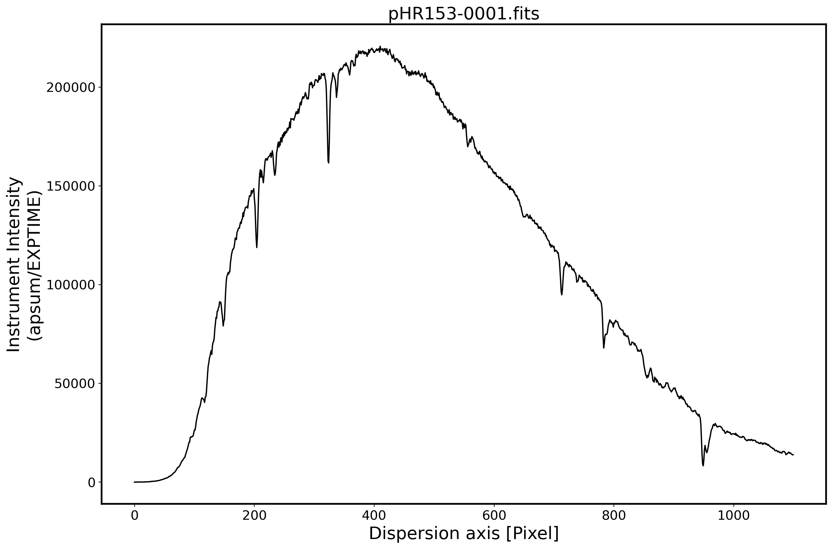
Aperture tracing & aperture sum for standard star#
# Bring the sample image

OBJECTNAME = SUBPATH/'pHR153-0001.fits'
hdul = fits.open(OBJECTNAME)[0]
obj = hdul.data
header = hdul.header
EXPTIME = header['EXPTIME']
fig,ax = plt.subplots(1,1,figsize=(10,15))
ax.imshow(obj,vmin=0,vmax=300)
ax.set_title('EXPTIME = {0}s'.format(EXPTIME))
ax.set_xlabel('Dispersion axis [pixel]')
ax.set_ylabel('Spatial axis \n [pixel]')
Text(0, 0.5, 'Spatial axis \n [pixel]')
# Let's find the peak along the spatial axis

# Plot the spectrum along the spatial direction
lower_cut = 700
upper_cut = 750
apall_1 = np.sum(obj[:,lower_cut:upper_cut],axis=1)

fig, ax = plt.subplots(1,1,figsize=(6,6))
ax.plot(apall_1)
ax.set_xlabel('Pixel number (Spatial axis)')
ax.set_ylabel('Pixel value')
ax.grid(ls=':')

# Find the peak

peak_pix = peak_local_max(apall_1, num_peaks=10,
                          min_distance=30,
                          threshold_abs=np.median(apall_1))
peak_pix = np.array(peak_pix[:,0])
print(peak_pix)

fig,ax = plt.subplots(1,1,figsize=(6,6))
x = np.arange(0, len(apall_1))
ax.plot(x, apall_1)
ax.set_xlabel('Spatial axis')

peak_value = []
for i in peak_pix:
    ax.plot((i, i),
            (apall_1[i]+0.01*max(apall_1),apall_1[i]+0.1*max(apall_1)),
            color='r', ls='-', lw=1)
    ax.annotate(i, (i, apall_1[i]+0.1*max(apall_1)),
            fontsize='small', rotation=45)
    peak_value.append(apall_1[i])
    print(i)

peak_pix = np.sort(peak_pix)

ax.grid(ls=':')
ax.set_xlabel('Pixel number (Spatial axis)')
ax.set_ylabel('Pixel value')

plt.show()

print(f'Pixel coordinatate in spatial direction = {peak_pix}')
[126]
126
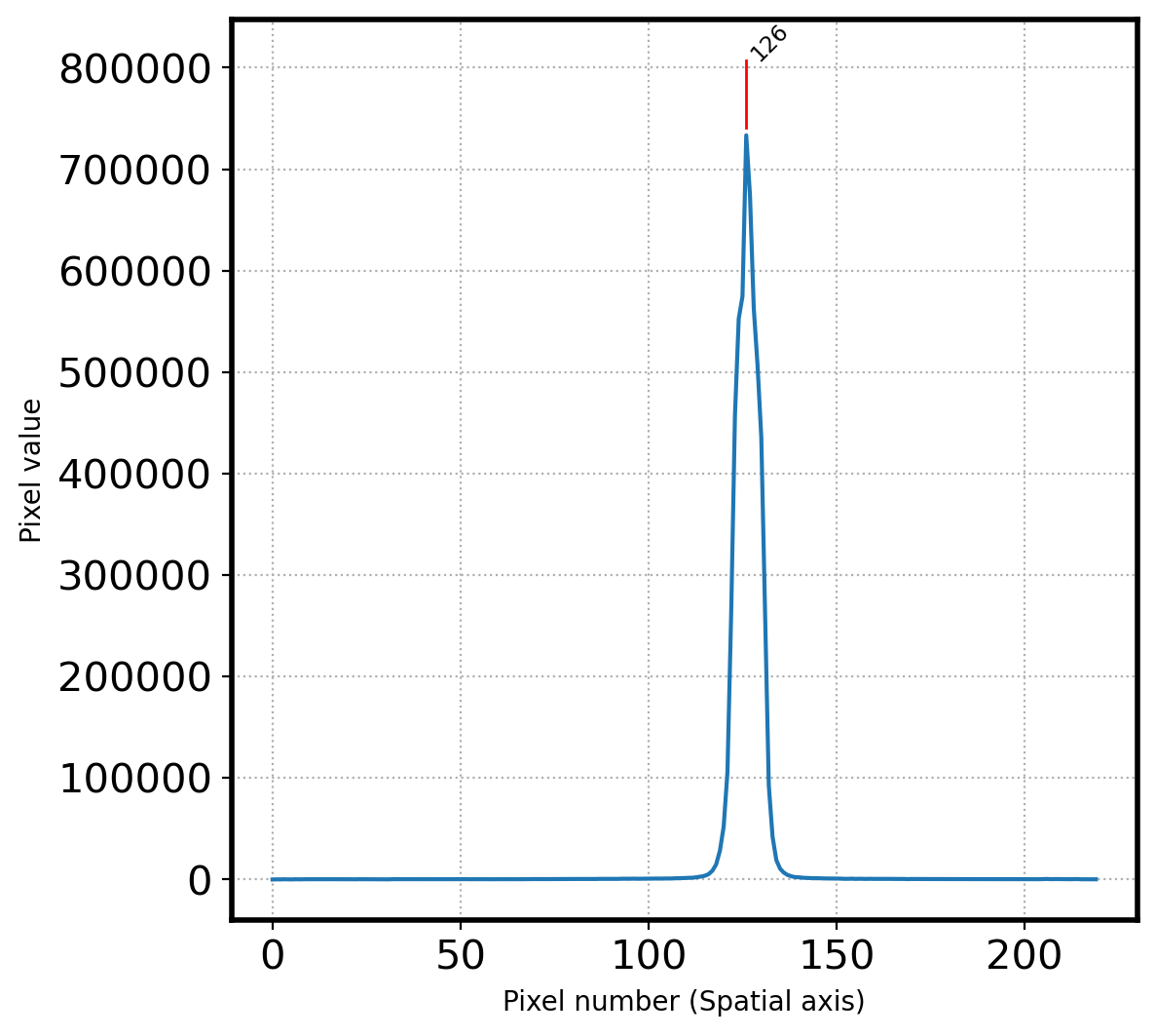
Pixel coordinatate in spatial direction = [126]
# Select the sky area
peak = peak_pix[0] # center
print('Peak pixel is {0} pix'.format(peak_pix[0]))

SKYLIMIT = 15 # pixel limit around the peak
RLIMIT = 10 # pixel limit from the rightmost area
LLIMIT = 10 # pixel limit from the leftmost area

mask_sky = np.full_like(x, True, dtype=bool)
for p in peak_pix:
    mask_sky[(x > p-SKYLIMIT) & (x < p+SKYLIMIT)] = False
mask_sky[:LLIMIT] = False
mask_sky[-RLIMIT:] = False

x_sky = x[mask_sky]
sky_val = apall_1[mask_sky]

# Plot the sky area
fig = plt.figure(figsize=(8, 5))
ax = fig.add_subplot(111)
ax.plot(x, apall_1, lw=1)
ax.fill_between(x, 0, 1, where=mask_sky, alpha=0.1, transform=ax.get_xaxis_transform())

ax.set_xlabel('Pixel number')
ax.set_ylabel('Pixel value sum')
Peak pixel is 126 pix
Text(0, 0.5, 'Pixel value sum')
# Sigma clipping
Sigma = 3
clip_mask = sigma_clip(sky_val,
                       sigma=Sigma,
                       maxiters= 5).mask

# Fit the sky
ORDER_APSKY = 3
coeff_apsky, fitfull = chebfit(x_sky[~clip_mask],
                               sky_val[~clip_mask],
                               deg=ORDER_APSKY,
                               full=True)
sky_fit = chebval(x, coeff_apsky)

# Calculate the RMS of Fit
residual = fitfull[0][0]
fitRMS = np.sqrt(residual/len(x_sky[~clip_mask]))


n_sky = len(x_sky)
n_rej = np.count_nonzero(clip_mask)

# Plot the sky area & fitted sky
fig,ax = plt.subplots(1,1,figsize=(8, 5))

ax.plot(x, apall_1, lw=1)
ax.plot(x, sky_fit, ls='--',
        label='Sky Fit ({:d}/{:d} used)'.format(n_sky - n_rej, n_sky))
ax.plot(x_sky[clip_mask], sky_val[clip_mask], marker='x', ls='', ms=10)
ax.fill_between(x, 0, 1, where=mask_sky, alpha=0.1, transform=ax.get_xaxis_transform())


title_str = r'Skyfit: {:s} order {:d} ({:.1f}-sigma {:d}-iters)'
ax.set_xlabel('Pixel number')
ax.set_ylabel('Pixel value sum')
ax.legend()
ax.set_title(title_str.format('Chebyshev', ORDER_APSKY,
                              Sigma, 5))
Text(0.5, 1.0, 'Skyfit: Chebyshev order 3 (3.0-sigma 5-iters)')
# Finding the peak center by fitting the gaussian 1D function again

sub_apall_1 = apall_1 - sky_fit # profile - sky

# OUTPIX = 50 # number of pixels to rule out outermost area in spacial direction
# xx = x[OUTPIX:-OUTPIX]
# yy = sub_apall_1[OUTPIX:-OUTPIX]

xx = x[peak-SKYLIMIT:peak+SKYLIMIT]
yy = sub_apall_1[peak-SKYLIMIT:peak+SKYLIMIT]

# gaussian modeling
g_init = Gaussian1D(amplitude=sub_apall_1[peak],
                    mean=peak,
                    stddev=15*gaussian_fwhm_to_sigma)

fitter = LevMarLSQFitter()
fitted = fitter(g_init, xx, yy)

params = [fitted.amplitude.value, fitted.mean.value, fitted.stddev.value]

fig = plt.figure()
ax = fig.add_subplot(111)
x = np.arange(0, len(apall_1))
ax.plot(x, sub_apall_1, label='Spatial profile')

g = Gaussian1D(*params)

ax.plot(x, g(x), label='Fitted 1D Gaussian profile')
ax.grid(ls=':')
ax.set_xlabel('Pixel number (Spatial axis)')
ax.set_ylabel('Pixel value')
ax.set_ylim(0, sub_apall_1[peak])
ax.legend(loc=2,fontsize=10)
plt.show()

center_pix = params[1]
print('center pixel:', center_pix)
center pixel: 126.3998688552938
# Trace the aperture (peak) along the wavelength.
# Repeat the above process for all wavelength bands.
# This process is called "aperture tracing".
aptrace = []
aptrace_fwhm = []
STEP_AP = 10
N_AP = len(obj[0])//STEP_AP
FWHM_AP = 10
peak = center_pix
for i in range(N_AP - 1):
    lower_cut, upper_cut = i*STEP_AP, (i+1)*STEP_AP
    apall_i = np.sum(obj[:, lower_cut:upper_cut], axis=1)
    sky_val = apall_i[mask_sky]
    clip_mask = sigma_clip(sky_val,
                           sigma=3,
                           maxiters=5).mask
    coeff, fitfull = chebfit(x_sky[~clip_mask],
                             sky_val[~clip_mask],
                             deg=ORDER_APSKY,
                             full=True)
    apall_i -= chebval(x,coeff)  # Object profile - the fitted sky

    search_min = int(peak - 3*FWHM_AP)
    search_max = int(peak + 3*FWHM_AP)
    cropped = apall_i[search_min:search_max]
    x_cropped = np.arange(len(cropped))

    peak_pix_trace = peak_local_max(cropped,
                              min_distance=FWHM_AP,
                              num_peaks=1)
    peak_pix_trace = np.array(peak_pix_trace[:,0])

    if len(peak_pix_trace) == 0: # return NaN (Not a Number) if there is no peak found.
        aptrace.append(np.nan)
        aptrace_fwhm.append(0)
    else:
        peak_pix_trace = np.sort(peak_pix_trace)
        peak_trace = peak_pix_trace[0]
        g_init = Gaussian1D(amplitude=cropped[peak_trace], # Gaussian fitting to find centers
                            mean=peak_trace,
                            stddev=FWHM_AP*gaussian_fwhm_to_sigma,
                            bounds={'amplitude':(0, 2*cropped[peak_trace]) ,
                                    'mean':(peak_trace-3*FWHM_AP, peak_trace+3*FWHM_AP),
                                    'stddev':(0.00001, FWHM_AP*gaussian_fwhm_to_sigma)})
        fitted = fitter(g_init, x_cropped, cropped)
        center_pix_new = fitted.mean.value + search_min
        aptrace_fwhm.append(fitted.fwhm)
        aptrace.append(center_pix_new)

aptrace = np.array(aptrace)
aptrace_fwhm = np.array(aptrace_fwhm)
# Plot the center of profile peak
fig,ax = plt.subplots(2,1,figsize=(10,5))
ax[0].imshow(obj,vmin=0,vmax=300)
ax[0].set_xlabel('Dispersion axis',fontsize=15)
ax[0].set_ylabel('Spatial axis',fontsize=15)
xlim = ax[0].get_xlim()

ax[1].plot(np.arange(len(aptrace))*10, aptrace,ls='', marker='+', ms=10,color='lightskyblue')
ax[1].set_xlim(xlim)
ax[1].set_ylim(200,0) # you can see the jiggly-wiggly shape when you zoom in
ax[1].set_xlabel('Dispersion axis',fontsize=15)
ax[1].set_ylabel('Spatial axis',fontsize=15)
Text(0, 0.5, 'Spatial axis')
# Fitting the peak with Chebyshev function

ORDER_APTRACE = 9
SIGMA_APTRACE = 3
ITERS_APTRACE = 5 # when sigma clipping

# Fitting the line
x_aptrace = np.arange(N_AP-1) * STEP_AP
coeff_aptrace = chebfit(x_aptrace, aptrace, deg=ORDER_APTRACE)

# Sigma clipping
resid_mask = sigma_clip(aptrace - chebval(x_aptrace, coeff_aptrace),
                        sigma=SIGMA_APTRACE, maxiters=ITERS_APTRACE).mask

# Fitting the peak again after sigma clipping
x_aptrace_fin = x_aptrace[~resid_mask]
aptrace_fin = aptrace[~resid_mask]
coeff_aptrace_fin = chebfit(x_aptrace_fin, aptrace_fin, deg=ORDER_APTRACE)

fit_aptrace_fin   = chebval(x_aptrace_fin, coeff_aptrace_fin)
resid_aptrace_fin = aptrace_fin - fit_aptrace_fin
del_aptrace = ~np.in1d(x_aptrace, x_aptrace_fin) # deleted points #x_aptrace에서 x_aptrace_fin이 없으면 True
'''
test = np.array([0, 1, 2, 5, 0])
states = [0, 2]
mask = np.in1d(test, states)
mask
array([ True, False,  True, False,  True])
'''


# Plot the Fitted line & residual
fig = plt.figure(figsize=(10,8))
gs = gridspec.GridSpec(3, 1)
ax1 = plt.subplot(gs[0:2])
ax2 = plt.subplot(gs[2])

ax1.plot(x_aptrace, aptrace, ls='', marker='+', ms=10,color='lightskyblue')
ax1.plot(x_aptrace_fin, fit_aptrace_fin, ls='--',color='crimson',zorder=10,lw=2,
         label="Aperture Trace ({:d}/{:d} used)".format(len(aptrace_fin), N_AP-1))
ax1.plot(x_aptrace[del_aptrace], aptrace[del_aptrace], ls='', marker='x',color='salmon', ms=10)
ax1.set_ylabel('Found object position')
ax1.grid(ls=':')
ax1.legend()


ax2.plot(x_aptrace_fin, resid_aptrace_fin, ls='', marker='+')
ax2.axhline(+np.std(resid_aptrace_fin, ddof=1), ls=':', color='k')
ax2.axhline(-np.std(resid_aptrace_fin, ddof=1), ls=':', color='k',
            label='residual std')


ax2.set_ylabel('Residual (pixel)')
ax2.set_xlabel('Dispersion axis (pixel)')

ax2.grid(ls=':')
ax2.set_ylim(-3, 3)
ax2.legend()

#Set plot title
title_str = ('Aperture Trace Fit ({:s} order {:d})\n'
            + 'Residuials {:.1f}-sigma, {:d}-iters clipped')
plt.suptitle(title_str.format('Chebshev', ORDER_APTRACE,
                              SIGMA_APTRACE, ITERS_APTRACE))
plt.show()
# Aperture sum

apsum_sigma_lower = 3 # [Sigma]
apsum_sigma_upper = 3
ap_fwhm = np.median(aptrace_fwhm[~resid_mask]) # [pix]
ap_sigma = ap_fwhm * gaussian_fwhm_to_sigma # [pixel/sigma]
x_ap = np.arange(len(obj[0])) # pixel along the dispersion axis
y_ap = chebval(x_ap, coeff_aptrace_fin) # center of peak for each line

# Extract the spectrum along the dispersion axis
ap_summed  = []
ap_sig = []

for i in range(len(obj[0])):
    cut_i = obj[:,i] # Cut spatial direction
    peak_i = y_ap[i]
    offset_i = peak_i - peak

    mask_sky_i = np.full_like(x, True, dtype=bool)
    for p in peak_pix:
        mask_sky_i[(x > p+offset_i-SKYLIMIT) & (x < p+offset_i+SKYLIMIT)] = False
    mask_sky_i[:LLIMIT] = False
    mask_sky_i[-RLIMIT:] = False

    # aperture size = apsum_sigma_lower * ap_sigma
    x_obj_lower = int(np.around(peak_i - apsum_sigma_lower * ap_sigma))
    x_obj_upper = int(np.around(peak_i + apsum_sigma_upper * ap_sigma))
    x_obj = np.arange(x_obj_lower, x_obj_upper)
    obj_i = cut_i[x_obj_lower:x_obj_upper]

    # Fitting Sky value
    x_sky = x[mask_sky_i]
    sky_val = cut_i[mask_sky_i]
    clip_mask = sigma_clip(sky_val, sigma=Sigma,
                           maxiters=5).mask
    coeff = chebfit(x_sky[~clip_mask],
                    sky_val[~clip_mask],
                    deg=ORDER_APSKY)

    # Subtract the sky
    sub_obj_i = obj_i - chebval(x_obj, coeff) # obj - lsky  subtraction


    # Calculate error
    sig_i = RN **2 + sub_obj_i + chebval(x_obj,coeff)
    # RN**2 + flux_i + sky value

    ap_summed.append(np.sum(sub_obj_i))
    ap_sig.append(np.sqrt(np.sum(sig_i)))

ap_summed = np.array(ap_summed) / EXPTIME
ap_std = np.array(ap_sig) / EXPTIME
# Plot the spectrum

x_pix = np.arange(len(obj[0]))

fig,ax = plt.subplots(1,1,figsize=(15,10))
ax.plot(x_pix,ap_summed,color='k',alpha=1)


FILENAME = OBJECTNAME.name
ax.set_title(FILENAME,fontsize=20)
ax.set_ylabel('Instrument Intensity\n(apsum/EXPTIME)',fontsize=20)
ax.set_xlabel(r'Dispersion axis [Pixel]',fontsize=20)
ax.tick_params(labelsize=15)
plt.show()

spec_before_wfcali = Table([x_pix, ap_summed, ap_std],
                          names=['x_pix', 'ap_summed', 'ap_std'])


spec_before_wfcali.write(SUBPATH/(OBJECTNAME.stem+'_inst_spec.csv'),
                        overwrite=True, format='csv')
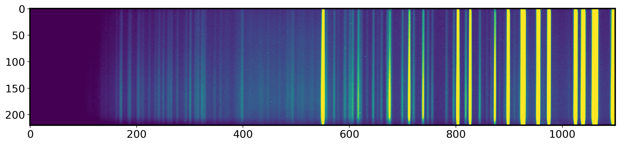
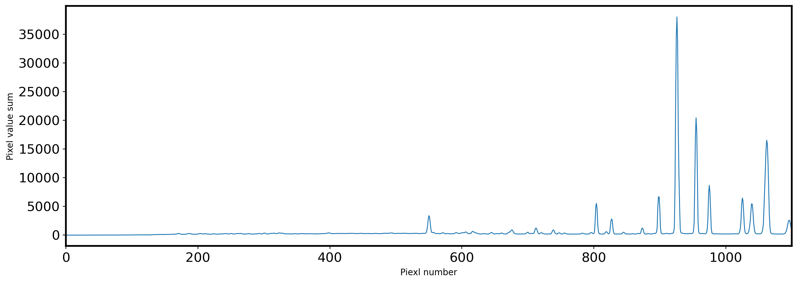
2-2. Wavelength calibration#
# Bring the Master Comparison image
Master_comparison = SUBPATH/'pMaster_Neon.fits'
compimage = fits.open(Master_comparison)[0].data
identify = np.median(compimage[90:110,:],
                         axis=0)
fig,ax = fig,ax = plt.subplots(1,1,figsize=(15,5))
ax.imshow(compimage, vmin=0, vmax=1000)

fig,ax = plt.subplots(1,1,figsize=(15,5))
x_identify = np.arange(0,len(identify))
ax.plot(x_identify,identify,lw=1)
ax.set_xlabel('Piexl number')
ax.set_ylabel('Pixel value sum')
ax.set_xlim(0,len(identify))
plt.show()
plt.tight_layout()
<Figure size 640x480 with 0 Axes>
#Comparison Lampe line list

LISTFILE = SUBPATH/'neon1.gif'
Image(filename = LISTFILE, width=800)
#http://astrosurf.com/buil/us/spe2/hresol4.htm
---------------------------------------------------------------------------
FileNotFoundError                         Traceback (most recent call last)
/var/folders/c3/0f663kw90xldstvklyr5nq9c0000gn/T/ipykernel_20589/2335254067.py in <module>
      2
      3 LISTFILE = SUBPATH/'neon1.gif'
----> 4 Image(filename = LISTFILE, width=800)
      5 #http://astrosurf.com/buil/us/spe2/hresol4.htm

/opt/anaconda3/envs/main/lib/python3.9/site-packages/IPython/core/display.py in __init__(self, data, url, filename, format, embed, width, height, retina, unconfined, metadata)
   1229         self.retina = retina
   1230         self.unconfined = unconfined
-> 1231         super(Image, self).__init__(data=data, url=url, filename=filename,
   1232                 metadata=metadata)
   1233

/opt/anaconda3/envs/main/lib/python3.9/site-packages/IPython/core/display.py in __init__(self, data, url, filename, metadata)
    635             self.metadata = {}
    636
--> 637         self.reload()
    638         self._check_data()
    639

/opt/anaconda3/envs/main/lib/python3.9/site-packages/IPython/core/display.py in reload(self)
   1261         """Reload the raw data from file or URL."""
   1262         if self.embed:
-> 1263             super(Image,self).reload()
   1264             if self.retina:
   1265                 self._retina_shape()

/opt/anaconda3/envs/main/lib/python3.9/site-packages/IPython/core/display.py in reload(self)
    660         """Reload the raw data from file or URL."""
    661         if self.filename is not None:
--> 662             with open(self.filename, self._read_flags) as f:
    663                 self.data = f.read()
    664         elif self.url is not None:

FileNotFoundError: [Errno 2] No such file or directory: '/Users/hbahk/class/ao22/SNU_AO22-2/_test/data/neon1.gif'
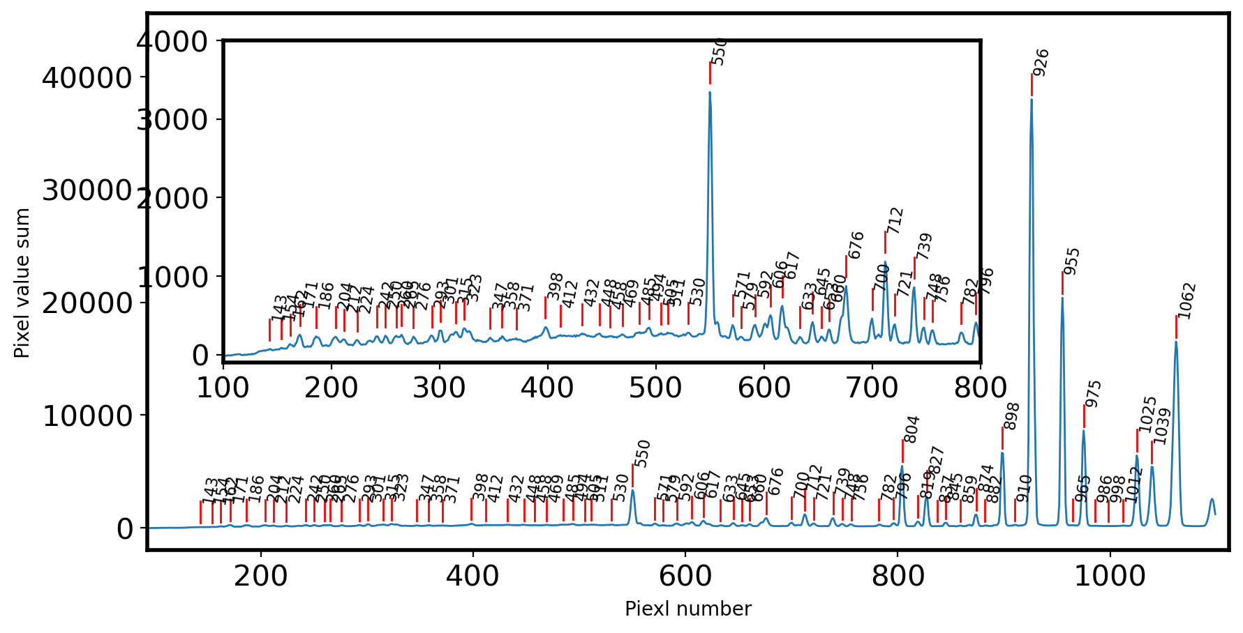
# Find the local peak

peak_pix = peak_local_max(identify,
                          num_peaks=max(identify),
                          min_distance=4,
                          threshold_abs=max(identify)*0.001)

fig,ax = plt.subplots(1, 1, figsize=(10, 5))
x_identify = np.arange(0, len(identify))
ax.plot(x_identify, identify, lw=1)
for i in peak_pix:
    ax.plot([i, i],
            [identify[i]+0.01*max(identify), identify[i]+0.06*max(identify)],
            color='r',lw=1)
    ax.annotate(i[0], (i, identify[i]+0.06*max(identify)),
                fontsize=8,
                rotation=80)

ax.set_xlabel('Piexl number')
ax.set_ylabel('Pixel value sum')
ax.set_xlim(min(peak_pix)[0] - 50,max(peak_pix)[0] + 50)
ax.set_ylim(-2000, max(identify) + max(identify)*0.2)

axins = ax.inset_axes([0.07, 0.35, 0.7, 0.6])
axins.plot(x_identify, identify, lw=1)
axins.set_xlim(100, 800)
axins.set_ylim(-100, 4000)
for i in peak_pix:
    axins.plot([i, i],
            [identify[i]+0.003*max(identify), identify[i]+0.01*max(identify)],
            color='r', lw=1)
    axins.annotate(i[0],(i,identify[i]+0.01*max(identify)),
                fontsize=8,
                rotation=80)

plt.show()
plt.tight_layout()
<Figure size 640x480 with 0 Axes>
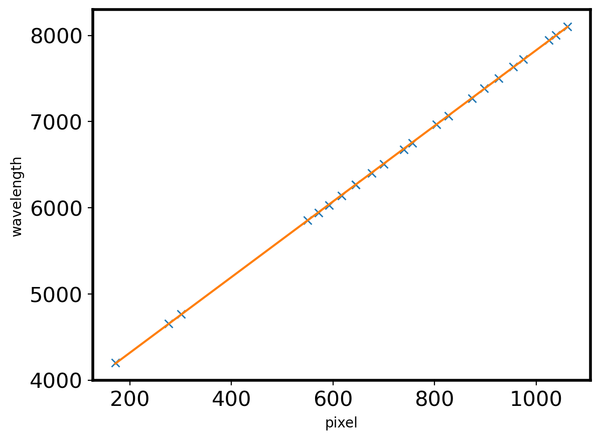
# Find the matching pair of wavelength and pixel
pixel_init, wavelength = np.array([
                                    [171,  4200.674],
                                    [276,  4657.901],
                                    [301,  4764.865],
                                    # [739,  6677.282],
                                    [550,  5852.488], # Ne
                                    [571,  5944.834], # Ne
                                    [592,  6029.997], # Ne
                                    [617,  6143.063], # Ne
                                    [645,  6266.495], # Ne
                                    [676,  6402.246], # Ne
                                    [700,  6506.528], # Ne
                                    [739,  6678.276], # Ne
                                    [756,  6752.834],
                                    [804,  6965.431],
                                    [827,  7067.218],
                                    [874,  7272.936],
                                    [898,  7383.980],
                                    [926,  7503.869],
                                    [955,  7635.106],
                                    [975,  7724.207],
                                    [1025, 7948.176],
                                    [1039, 8006.157],
                                    [1062, 8103.693],
                                   ]).T

ID_init = dict(pixel_init=pixel_init.astype('int'), wavelength=wavelength)

ID_init = Table(ID_init)
plt.plot(ID_init['pixel_init'],ID_init['wavelength'],marker='x',ls='')

def linear(x,a,b):
    return a*x + b
popt,pcov = curve_fit(linear,ID_init['pixel_init'],ID_init['wavelength'])
plt.plot(ID_init['pixel_init'],linear(ID_init['pixel_init'],*popt))
plt.xlabel('pixel')
plt.ylabel('wavelength')
print(linear(550,*popt))
5853.743449933852
# Fit the each peak with Gaussian 1D function

peak_gauss = []
fitter = LevMarLSQFitter()
LINE_FITTER = LevMarLSQFitter()
FWHM_ID = 3
x_identify = np.arange(0,len(identify))

# Gaussian fitting for each peak (pixel)
for peak_pix in ID_init['pixel_init']:
    g_init = Gaussian1D(amplitude=identify[peak_pix],
                        mean = peak_pix,
                        stddev = FWHM_ID*gaussian_fwhm_to_sigma,
                        bounds={'amplitude':(0,2*identify[peak_pix]),
                                'mean':(peak_pix - FWHM_ID,peak_pix + FWHM_ID),
                                'stddev':(0,FWHM_ID)})
    fitted = LINE_FITTER(g_init,x_identify,identify) #Model, x, y
    peak_gauss.append(fitted.mean.value)
    print(peak_pix,'->',fitted.mean.value)


peak_gauss = Column(data=peak_gauss,
                        name='pixel_gauss',
                        dtype=float)
peak_shift = Column(data=peak_gauss - ID_init['pixel_init'],
                    name='piexl_shift',
                    dtype=float)
ID_init['pixel_gauss'] = peak_gauss
ID_init['pixel_shift'] = peak_gauss - ID_init['pixel_init']
ID_init.sort('wavelength')
ID_init.pprint()
171 -> 170.56957283749878
276 -> 275.92035369063353
301 -> 300.8979507517763
550 -> 550.2983570133845
571 -> 570.9150212096177
592 -> 593.4469235222318
617 -> 617.20066724794
645 -> 644.9814730829559
645 -> 644.9814730829559
676 -> 675.1637490708239
700 -> 700.2697277340493
739 -> 738.6514955795404
756 -> 755.1372254909968
804 -> 803.8969923950391
827 -> 826.969298371428
874 -> 873.5005033342331
898 -> 898.4810339834836
926 -> 925.9588245798751
955 -> 955.0558910850668
975 -> 975.0952675012696
1025 -> 1025.2927007263313
1039 -> 1039.5376383005416
1062 -> 1061.992030535472
pixel_init wavelength    pixel_gauss          pixel_shift
---------- ---------- ------------------ ---------------------
       171   4200.674 170.56957283749878   -0.4304271625012177
       276   4657.901 275.92035369063353    -0.079646309366467
       301   4764.865  300.8979507517763  -0.10204924822369321
       550   5852.488  550.2983570133845   0.29835701338447507
       571   5944.834  570.9150212096177  -0.08497879038225165
       592   6029.997  593.4469235222318    1.4469235222318275
       617   6143.063    617.20066724794    0.2006672479400322
       645   6266.495  644.9814730829559 -0.018526917044141555
       645   6266.495  644.9814730829559 -0.018526917044141555
       676   6402.246  675.1637490708239   -0.8362509291761171
       700   6506.528  700.2697277340493    0.2697277340492974
       739   6678.276  738.6514955795404   -0.3485044204595624
       756   6752.834  755.1372254909968   -0.8627745090032022
       804   6965.431  803.8969923950391  -0.10300760496090788
       827   7067.218   826.969298371428 -0.030701628572046502
       874   7272.936  873.5005033342331   -0.4994966657668556
       898    7383.98  898.4810339834836    0.4810339834835986
       926   7503.869  925.9588245798751  -0.04117542012488684
       955   7635.106  955.0558910850668    0.0558910850668326
       975   7724.207  975.0952675012696    0.0952675012696318
      1025   7948.176 1025.2927007263313    0.2927007263313044
      1039   8006.157 1039.5376383005416    0.5376383005416301
      1062   8103.693  1061.992030535472 -0.007969464528059689
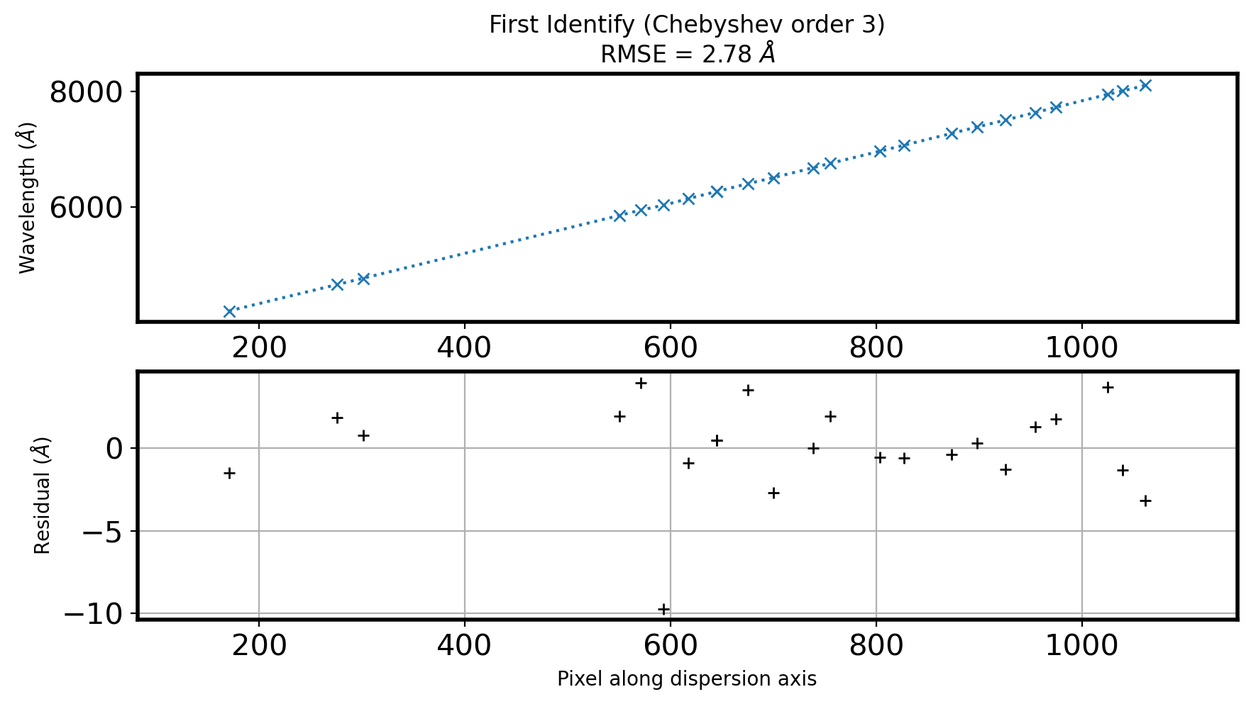
#Derive dispersion solution

ORDER_ID = 3 #Order of fitting function #보통 3 이하로 함. 기기의 사용파장대가 넓으면 4를 사용할때도 있음.
coeff_ID, fitfull = chebfit(ID_init['pixel_gauss'],
                           ID_init['wavelength'],
                           deg=ORDER_ID,
                           full=True)  #Derive the dispersion solution

fitRMS = np.sqrt(fitfull[0][0]/len(ID_init))
rough_error = ((max(ID_init['wavelength'])-min(ID_init['wavelength']))
               /(max(ID_init['pixel_gauss'])-min(ID_init['pixel_gauss'])))/2
residual = (ID_init['wavelength'] #wavelength from reference
            -chebval(ID_init['pixel_gauss'],coeff_ID)) #wavelength derived from fitting
res_range = np.max(np.abs(residual))

fig,ax = plt.subplots(2,1,figsize=(10,5))
ax[0].plot(ID_init['pixel_gauss'],
         ID_init['wavelength'],
         ls = ':',marker='x')
ax[1].plot(ID_init['pixel_gauss'],
          residual,
          ls='',marker='+',
          color='k')
max_ID_init = max(ID_init['pixel_gauss'])
min_ID_init = min(ID_init['pixel_gauss'])
fig_xspan = max_ID_init - min_ID_init
fig_xlim = np.array([min_ID_init, max_ID_init]) + np.array([-1,1])*fig_xspan*0.1
ax[1].set_xlim(fig_xlim)
ax[0].set_xlim(fig_xlim)
ax[0].set_ylabel(r'Wavelength ($\AA$)')
ax[1].set_ylabel(r'Residual ($\AA$)')
ax[1].set_xlabel('Pixel along dispersion axis')
ax[0].set_title('First Identify (Chebyshev order {:d})\n'.format(ORDER_ID)
              + r'RMSE = {:.2f} $\AA$'.format(fitRMS))
ax[1].grid()
plt.show()
fig,ax = fig,ax = plt.subplots(1,1,figsize=(15,5))
ax.imshow(compimage,vmin=0,vmax=1000)
<matplotlib.image.AxesImage at 0x7f956da2f670>
# REIDENTIFY

STEP_AP = 5 #Step size in pixel (dispersion direction)
STEP_REID = 10 #Step size in pixel (spatial direction)
N_SPATIAL,N_WAVELEN = np.shape(compimage) #(220, 2048)
N_REID = N_SPATIAL//STEP_REID #Spatial direction
N_AP = N_WAVELEN//STEP_AP #Dispersion direction
TOL_REID = 5 # tolerence to lose a line in pixels

ORDER_WAVELEN_REID = 3
ORDER_SPATIAL_REID = 3

line_REID = np.zeros((N_REID-1,len(ID_init))) #Make the empty array (height, width)
spatialcoord = np.arange(0,(N_REID-1)*STEP_REID,STEP_REID) + STEP_REID/2
# spatialcoord = array([  5.,  15.,  25.,  35.,  45.,  55.,  65.,  75.,  85.,  95., 105.,
#       115., 125., 135., 145., 155., 165., 175., 185., 195., 205.])


#Repeat we did above along the spatial direction
for i in range(0,N_REID-1):
    lower_cut = i*STEP_REID
    upper_cut = (i+1)*STEP_REID
    reidentify_i = np.sum(compimage[lower_cut:upper_cut,:],axis=0)

    peak_gauss_REID = []

    for peak_pix_init in ID_init['pixel_gauss']:
        search_min = int(np.around(peak_pix_init - TOL_REID))
        search_max = int(np.around(peak_pix_init + TOL_REID))
        cropped = reidentify_i[search_min:search_max]
        x_cropped = np.arange(len(cropped)) + search_min

        #Fitting the initial gauss peak by usijng Gausian1D
        Amplitude_init = np.max(cropped)
        mean_init = peak_pix_init
        stddev_init = 5*gaussian_fwhm_to_sigma
        g_init = Gaussian1D(amplitude = Amplitude_init,
                           mean = mean_init,
                           stddev = stddev_init,
                           bounds={'amplitude':(0, 2*np.max(cropped)) ,
                                 'stddev':(0, TOL_REID)})
        g_fit = fitter(g_init,x_cropped,cropped)
        fit_center = g_fit.mean.value
        if abs(fit_center - peak_pix_init) > TOL_REID: #스펙트럼 끝에서는 잘 안 잡힐수있으니까
            peak_gauss_REID.append(np.nan)
            continue
        else:
            peak_gauss_REID.append(fit_center)

    peak_gauss_REID = np.array(peak_gauss_REID)
    nonan_REID = np.isfinite(peak_gauss_REID)
    line_REID[i,:] = peak_gauss_REID
    peak_gauss_REID_nonan = peak_gauss_REID[nonan_REID]
    n_tot = len(peak_gauss_REID)
    n_found = np.count_nonzero(nonan_REID)
    coeff_REID1D, fitfull = chebfit(peak_gauss_REID_nonan,
                                    ID_init['wavelength'][nonan_REID],
                                    deg=ORDER_WAVELEN_REID,
                                    full=True)
    fitRMS = np.sqrt(fitfull[0][0]/n_found)

points = np.vstack((line_REID.flatten(),
                    np.tile(spatialcoord, len(ID_init['pixel_init']))))
#np.tile(A,reps):Construct an array by repeating A the number of times given by reps.
# a = np.array([1, 2, 3])
# b = np.array([2, 3, 4])
# np.vstack((a,b)) = array([[1, 2, 3],[2, 3, 4]])
points = points.T # list of ()


values = np.tile(ID_init['wavelength'], N_REID - 1) #Wavelength corresponding to each point
values = np.array(values.tolist())  #
# errors = np.ones_like(values)


# #Fitting the wavelength along spatial direction and dispertion direction
coeff_init = Chebyshev2D(x_degree=ORDER_WAVELEN_REID, y_degree=ORDER_SPATIAL_REID)
fit2D_REID = fitter(coeff_init, points[:, 0], points[:, 1], values)
#Dispersion solution (both spatial & dispersion) #fitter(order,x,y,f(x,y))
WARNING: Model is linear in parameters; consider using linear fitting methods. [astropy.modeling.fitting]
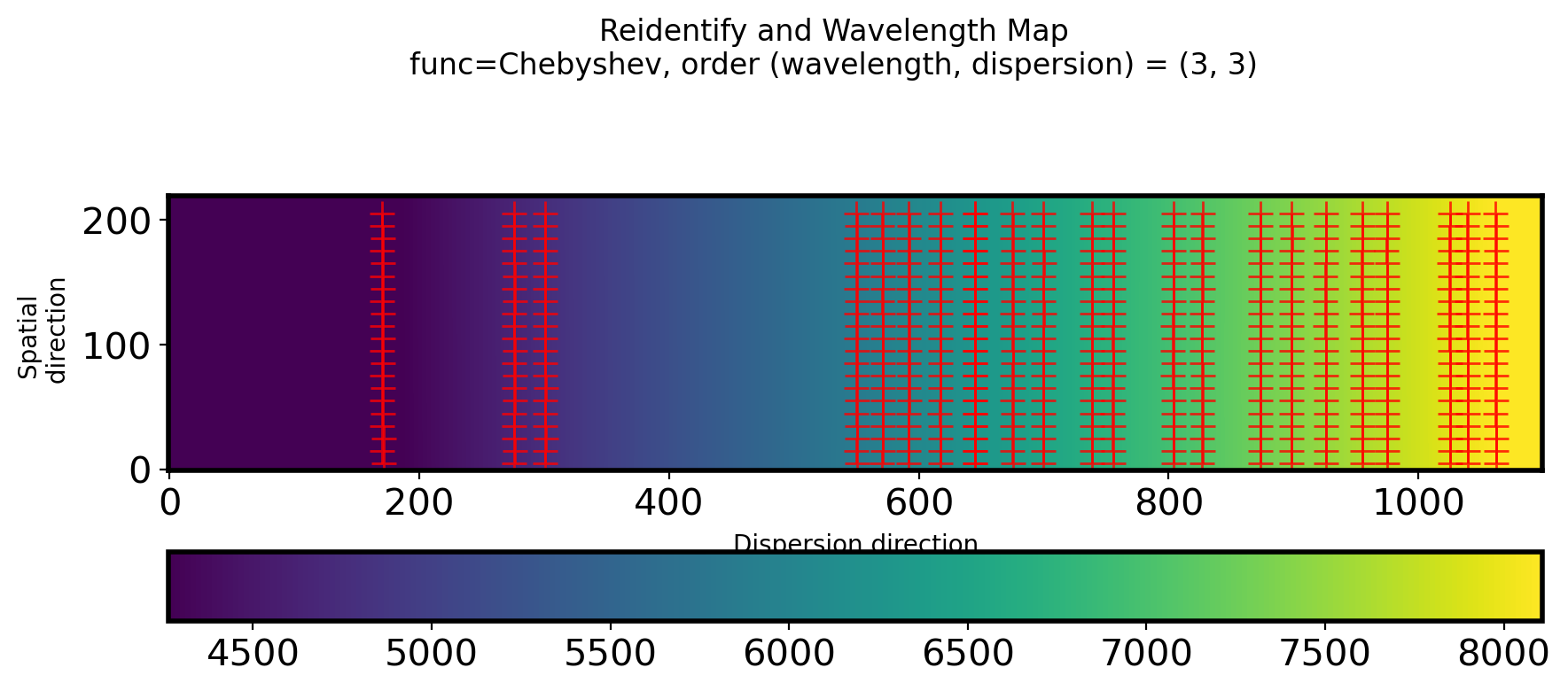
#Plot 2D wavelength callibration map and #Points to used re-identify
fig,ax = plt.subplots(1,1,figsize=(10,4))
ww, ss = np.mgrid[:N_WAVELEN, :N_SPATIAL]
im = ax.imshow(fit2D_REID(ww, ss).T, origin='lower',vmin=4264.4,vmax=8108.99)
ax.plot(points[:, 0], points[:, 1], ls='', marker='+', color='r',
alpha=0.8, ms=10)
fig.colorbar(im, ax=ax,orientation = 'horizontal')
ax.set_ylabel('Spatial \n direction')
ax.set_xlabel('Dispersion direction')
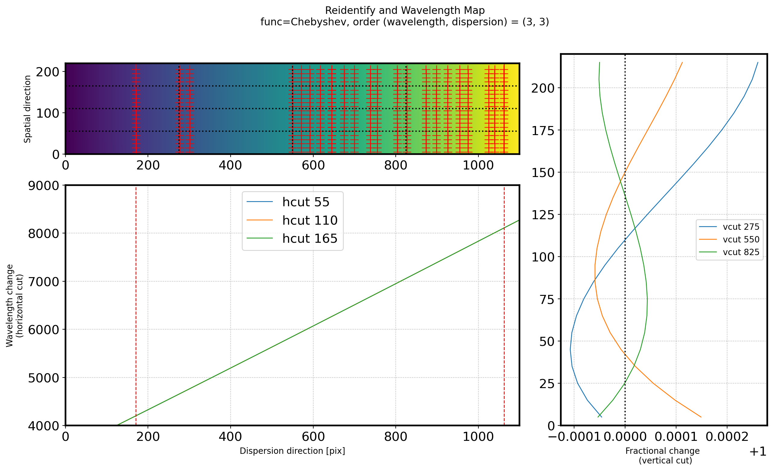
title_str = ('Reidentify and Wavelength Map\n'
+ 'func=Chebyshev, order (wavelength, dispersion) = ({:d}, {:d})')
plt.suptitle(title_str.format(ORDER_WAVELEN_REID, ORDER_SPATIAL_REID))
Text(0.5, 0.98, 'Reidentify and Wavelength Map\nfunc=Chebyshev, order (wavelength, dispersion) = (3, 3)')
# Check how the dispersion solution change along the spatial axis
# Divide spectrum into 4 equal parts in the spatial direction

fig,ax = plt.subplots(2,1,figsize=(10,7))
ax[0].imshow(fit2D_REID(ww, ss).T, origin='lower')
ax[0].plot(points[:, 0], points[:, 1], ls='', marker='+', color='r',
             alpha=0.8, ms=10)
# ax[0].set_xlim(0,2000)
ax[0].set_ylabel('Spatial \n direction')

title_str = ('Reidentify and Wavelength Map\n'
+ 'func=Chebyshev, order (wavelength, dispersion) = ({:d}, {:d}) \n')
plt.suptitle(title_str.format(ORDER_WAVELEN_REID, ORDER_SPATIAL_REID))


for i in (1, 2, 3):
    vcut = N_WAVELEN * i/4
    hcut = N_SPATIAL * i/4
    vcutax  = np.arange(0, N_SPATIAL, STEP_REID) + STEP_REID/2 #Spatial dir coordinate
    hcutax  = np.arange(0, N_WAVELEN, 1) # pixel along dispersion axis

    vcutrep = np.repeat(vcut, len(vcutax)) #i/4에 해당하는 dispersion pixel * len(spatial)
    hcutrep = np.repeat(hcut, len(hcutax)) #i/4에 해당하는 spatial pixel * len(dispersion)

    ax[0].axvline(x=vcut, ls=':', color='k')
    ax[0].axhline(y=hcut, ls=':', color='k')

    ax[1].plot(hcutax, fit2D_REID(hcutax, hcutrep), lw=1,
             label="horizon cut {:d} pix".format(int(hcut)))
# ax[1].set_xlim(0,2000)

ax[1].grid(ls=':')
ax[1].legend()
ax[1].set_xlabel('Dispersion direction')
ax[1].set_ylabel('Wavelength \n(horizontal cut)')
ax[1].set_ylim(min(ID_init['wavelength'])*0.5,max(ID_init['wavelength'])*1.5)


plt.tight_layout()
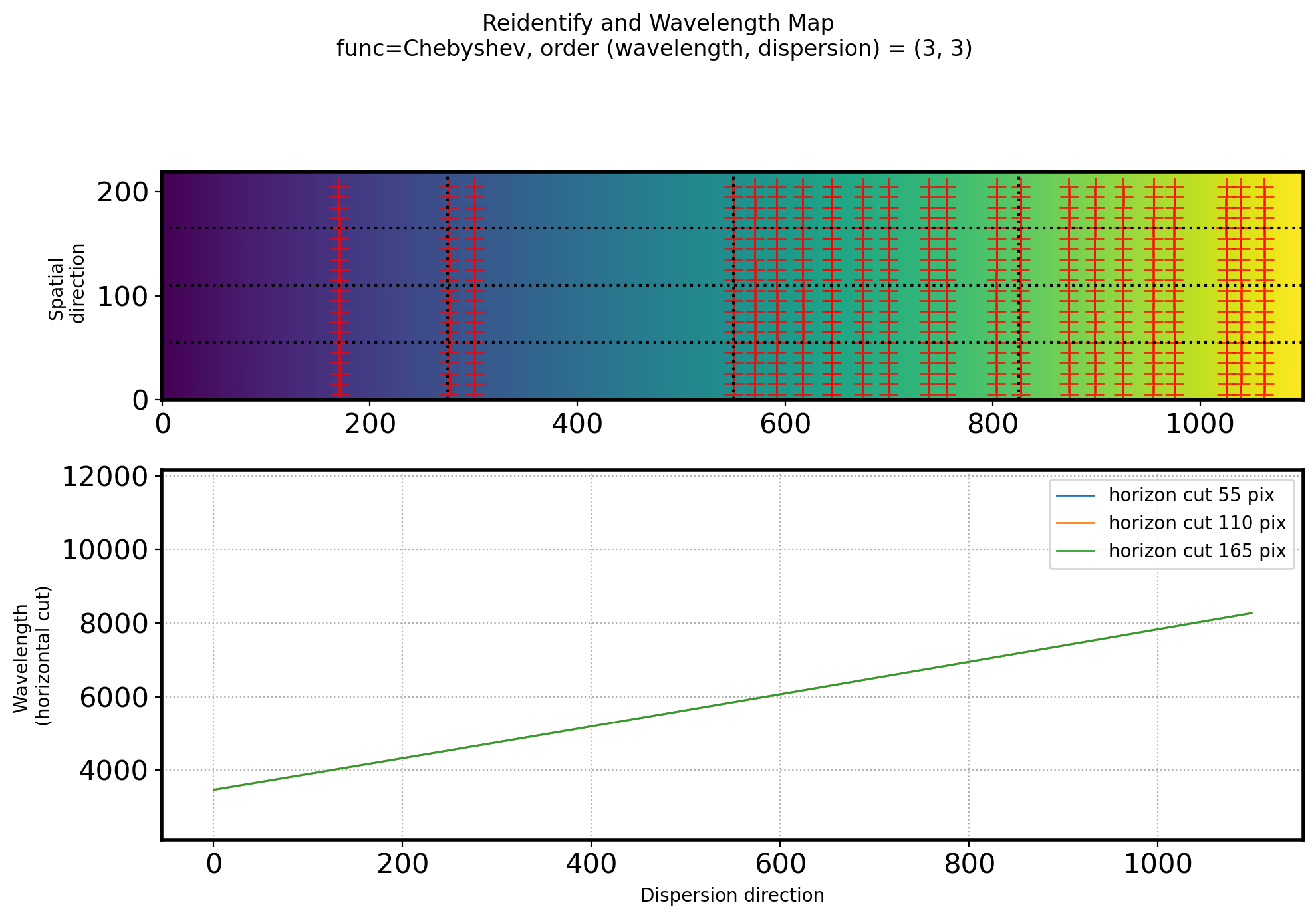
fig = plt.figure(figsize=(15, 8))
gs = gridspec.GridSpec(3, 3)
ax1 = plt.subplot(gs[:1, :2])
ax2 = plt.subplot(gs[1:3, :2])
ax3 = plt.subplot(gs[:3, 2])

# title
title_str = ('Reidentify and Wavelength Map\n'
             + 'func=Chebyshev, order (wavelength, dispersion) = ({:d}, {:d})')
plt.suptitle(title_str.format(ORDER_WAVELEN_REID, ORDER_SPATIAL_REID))


interp_min = line_REID[~np.isnan(line_REID)].min()
interp_max = line_REID[~np.isnan(line_REID)].max()

ax1.imshow(fit2D_REID(ww, ss).T, origin='lower')
ax1.axvline(interp_max, color='r', lw=1)
ax1.axvline(interp_min, color='r', lw=1)
ax1.plot(points[:, 0], points[:, 1], ls='', marker='+', color='r',
             alpha=0.8, ms=10)
ax1.set_xlim(0,2000)
ax1.set_ylabel('Spatial \n direction')


for i in (1, 2, 3):
    vcut = N_WAVELEN * i/4
    hcut = N_SPATIAL * i/4
    vcutax  = np.arange(0, N_SPATIAL, STEP_REID) + STEP_REID/2
    hcutax  = np.arange(0, N_WAVELEN, 1)
    vcutrep = np.repeat(vcut, len(vcutax))
    hcutrep = np.repeat(hcut, len(hcutax))

    ax1.axvline(x=vcut, ls=':', color='k')
    ax1.axhline(y=hcut, ls=':', color='k')

    ax2.plot(hcutax, fit2D_REID(hcutax, hcutrep), lw=1,
             label="hcut {:d}".format(int(hcut)))


    vcut_profile = fit2D_REID(vcutrep, vcutax)
    vcut_normalize = vcut_profile / np.median(vcut_profile)

    ax3.plot(vcut_normalize, vcutax, lw=1,
             label="vcut {:d}".format(int(vcut)))


ax2.axvline(interp_max, color='r', lw=1,ls='--')
ax2.axvline(interp_min, color='r', lw=1,ls='--')

ax1.set_ylabel('Spatial direction')
ax2.grid(ls=':')
ax2.legend(fontsize=15)
ax2.set_xlabel('Dispersion direction [pix]')
ax2.set_ylabel('Wavelength change\n(horizontal cut)')

ax3.axvline(1, ls=':', color='k')
ax3.grid(ls=':', which='both')
ax3.set_xlabel('Fractional change \n (vertical cut)')
ax3.legend(fontsize=10)

ax1.set_ylim(0, N_SPATIAL)
ax1.set_xlim(0, N_WAVELEN)
# ax2.set_xlim(300, 1700)
ax2.set_xlim(0, N_WAVELEN)
ax2.set_ylim(4000,9000)
ax3.set_ylim(0, N_SPATIAL)
plt.show()
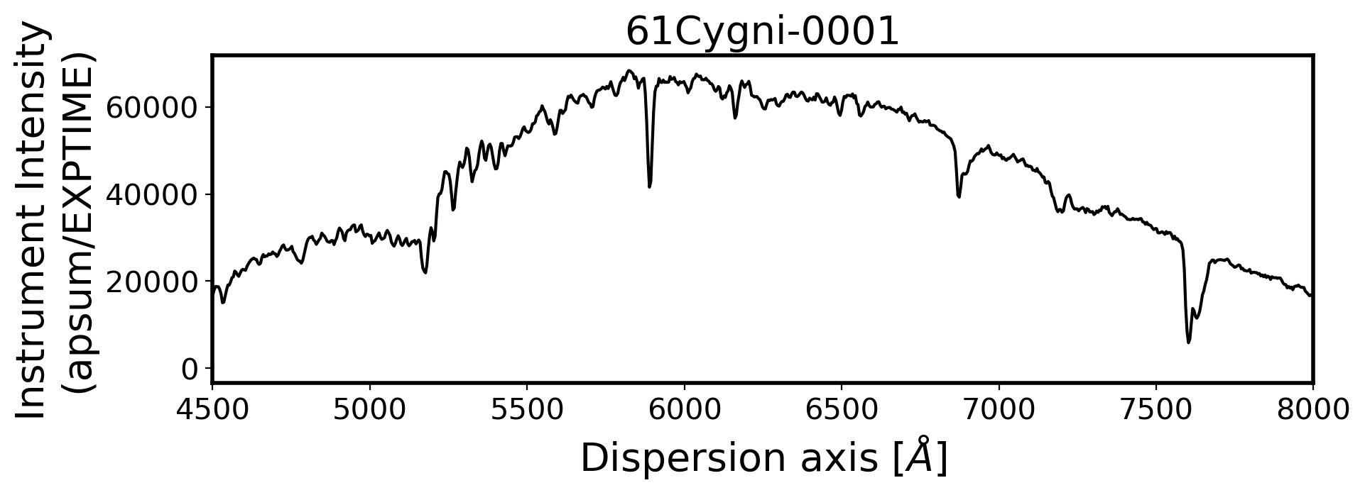
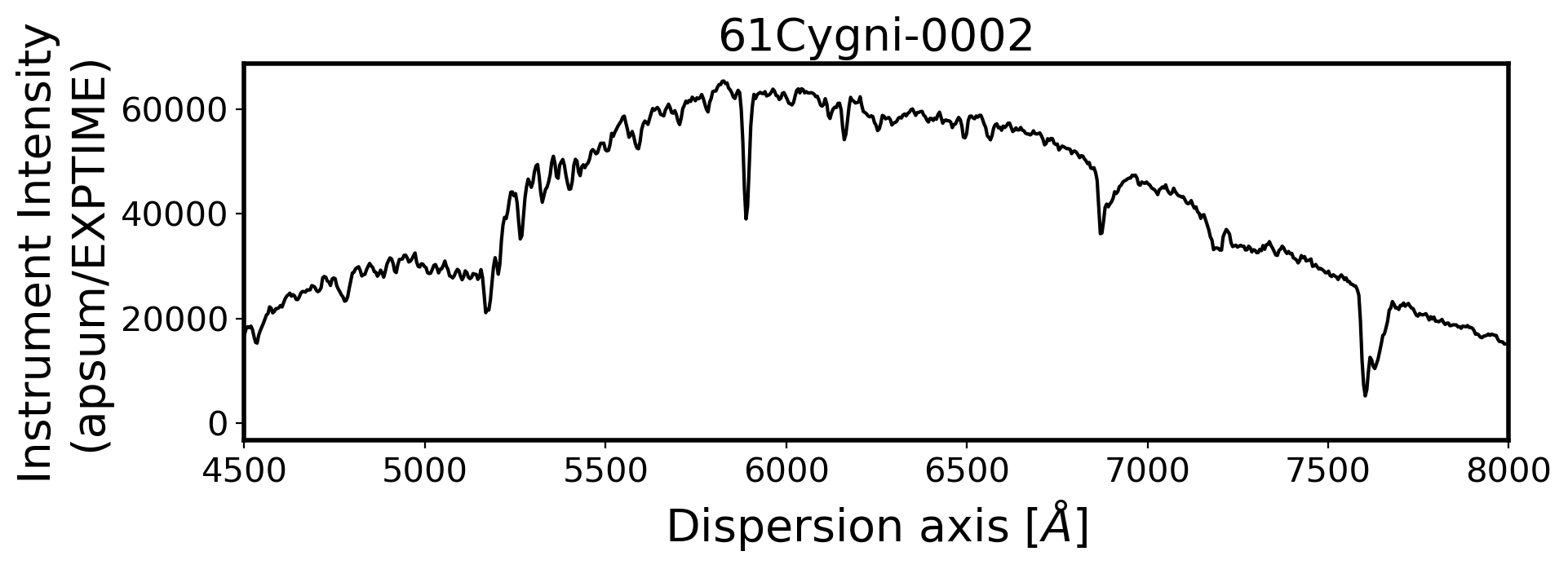
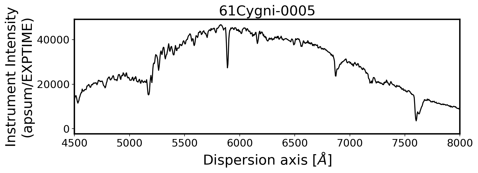
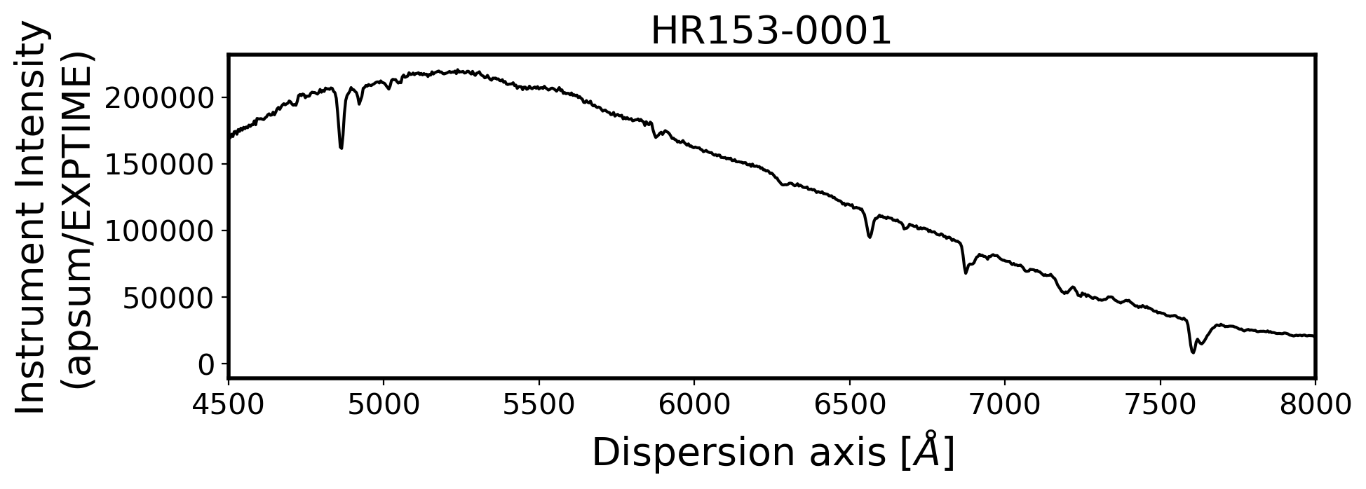
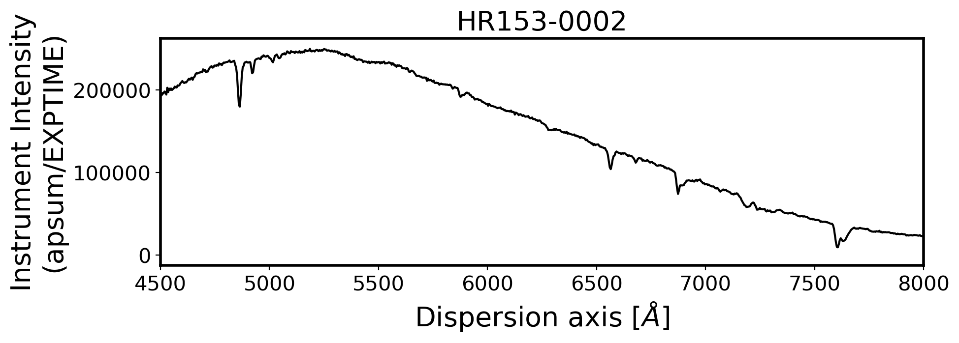
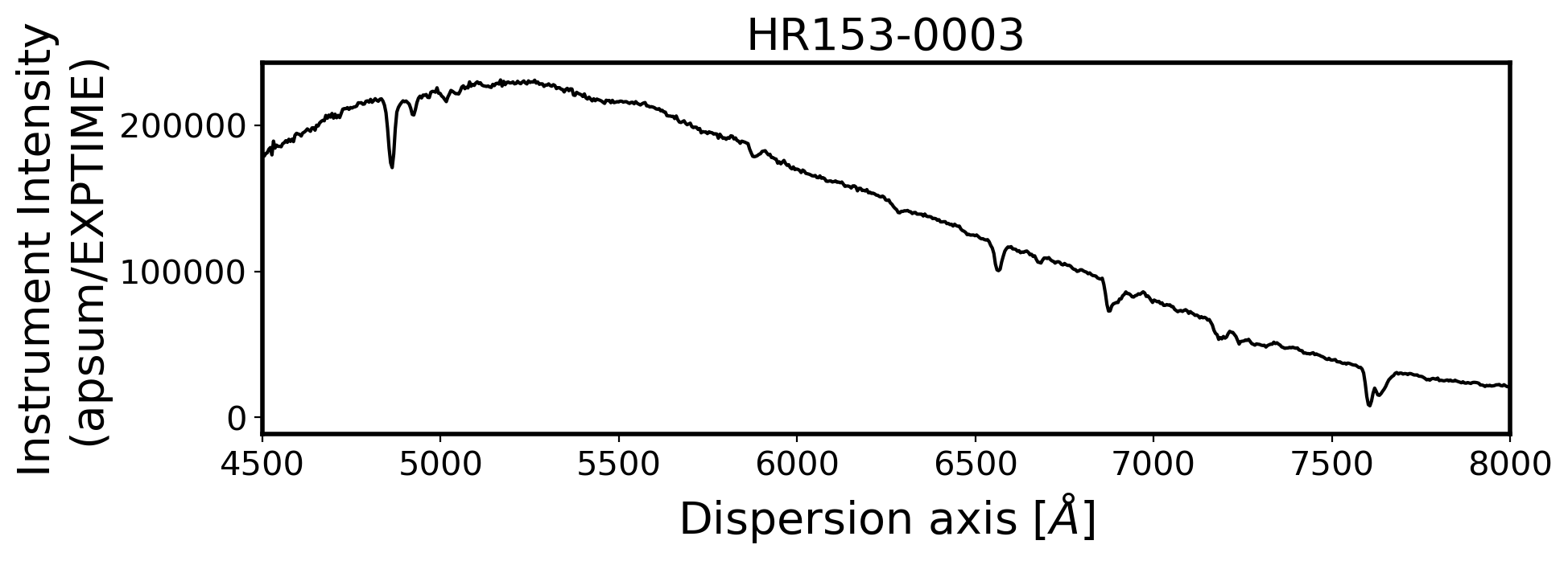
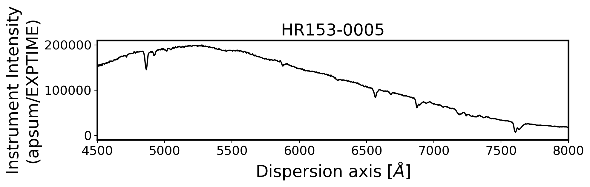
#Plot the spectrum respect to wavelength

Wavelength = chebval(np.arange(len(compimage[0])),coeff_ID)

x_pix = np.arange(len(obj[0]))


ObjStdList = Objectlist + Standlist
for i, path in enumerate(ObjStdList):
    fig, ax = plt.subplots(1,1,figsize=(10,3))
    OBJECTNAME = path.name
    FILENAME = path.stem
    obj = ascii.read(SUBPATH/('p'+FILENAME+'_inst_spec.csv'))
    ap_summed = obj['ap_summed']
    ap_std = obj['ap_std']
    ax.plot(Wavelength, ap_summed, color='k',alpha=1)
    ax.set_title(FILENAME, fontsize=20)
    ax.set_ylabel('Instrument Intensity\n(apsum/EXPTIME)', fontsize=20)
    ax.set_xlabel(r'Dispersion axis $[\AA]$', fontsize=20)
    ax.tick_params(labelsize=15)
    ax.set_xlim(4500, 8000)

    SAVE_FILENAME = SUBPATH/('p'+FILENAME+'_w_spec.csv')

    Data = [Wavelength, ap_summed, ap_std]
    data = Table(Data, names=['wave','inten','std'])
    data['wave'].format = "%.3f"
    data['inten'].format = "%.3f"
    data['std'].format = "%.3f"

    ascii.write(data, SAVE_FILENAME, overwrite=True, format='csv')

plt.tight_layout()


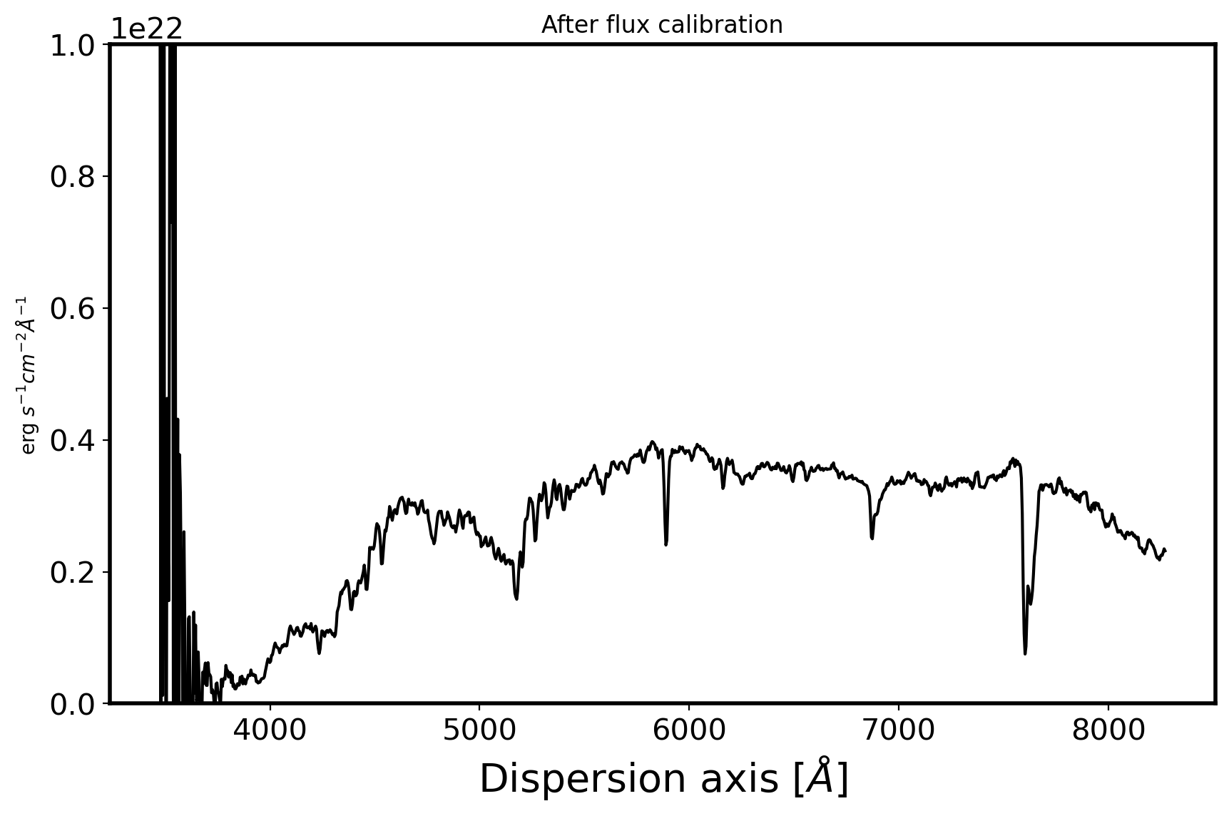
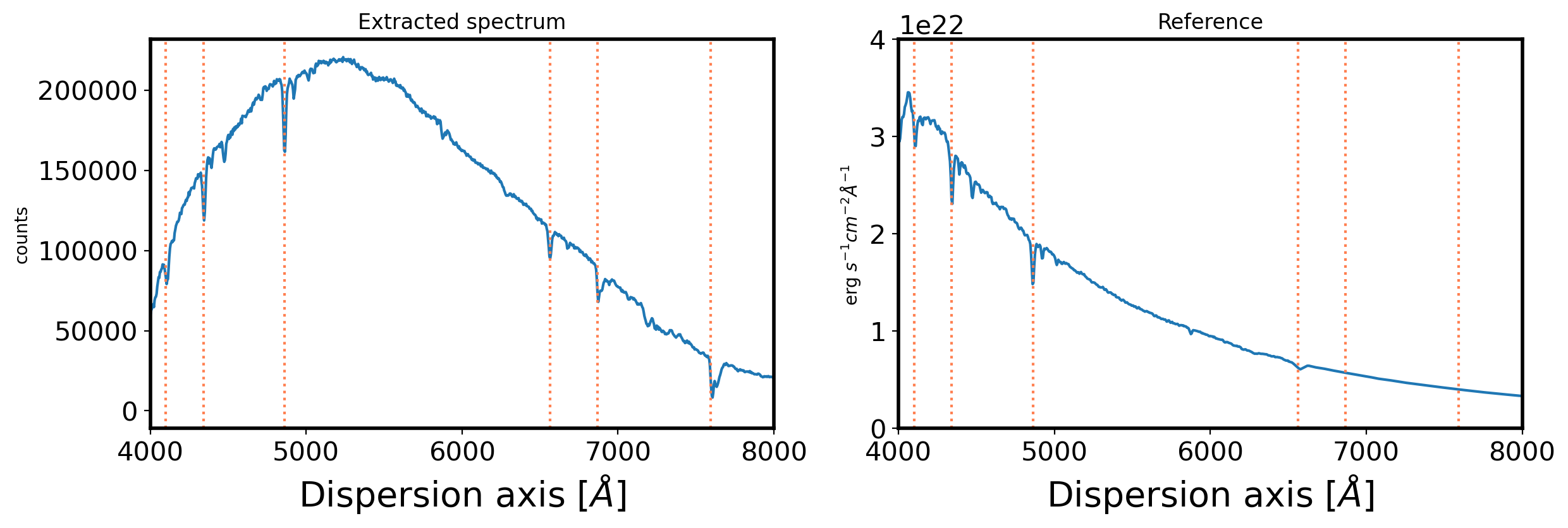
3. Flux calibration#
stdfile = SUBPATH/'fhr153.dat'
stddata = ascii.read(stdfile, names=['wave', 'flux', 'flux2'])
std_wave, std_flux  = stddata['wave'], stddata['flux']*1e16
std_wth = np.gradient(std_wave)

obj = ascii.read(SUBPATH/'pHR153-0001_w_spec.csv')
obj_wave = obj['wave']
obj_flux = obj['inten']

fig,ax = plt.subplots(1,2,figsize=(14,4))
ax[0].plot(obj_wave,obj_flux)
ax[0].set_xlim(4000,8000)
ax[0].set_title('Extracted spectrum')
ax[0].set_ylabel(r'counts')
ax[0].set_xlabel(r'Dispersion axis $[\AA]$',fontsize=20)
ax[1].plot(std_wave,std_flux)
ax[1].set_xlim(4000,8000)
ax[1].set_ylim(0, 0.4e23)
ax[1].set_title('Reference')
ax[1].set_ylabel(r'erg $s^{-1}cm^{-2}\AA^{-1}$ ')
ax[1].set_xlabel(r'Dispersion axis $[\AA]$',fontsize=20)

balmer = np.array([6563, 4861, 4341, 4100, 6867, 7593.7], dtype='float')
for i in balmer:
    ax[0].axvline(i,color='coral',ls=':')
    ax[1].axvline(i,color='coral',ls=':')
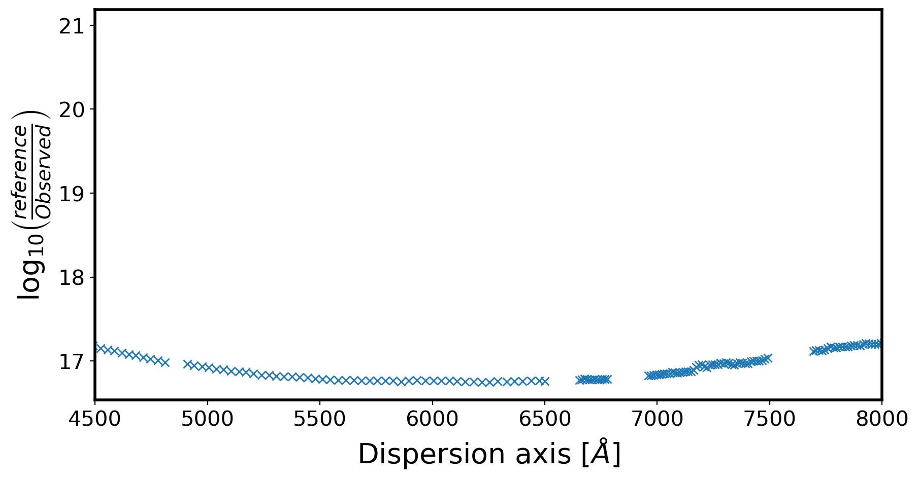
obj_flux_ds = []
obj_wave_ds = []
std_flux_ds = []

for i in range(len(std_wave)):
    rng = np.where((obj_wave >= std_wave[i] - std_wth[i] / 2.0) &
                           (obj_wave < std_wave[i] + std_wth[i] / 2.0)) #STD-wave 범위 안에 들어가는 obj_wave

    IsH = np.where((balmer >= std_wave[i] - 15*std_wth[i] / 2.0) &
                           (balmer < std_wave[i] + 15*std_wth[i] / 2.0))

    if (len(rng[0]) > 1) and (len(IsH[0]) == 0):
        # does this bin contain observed spectra, and no Balmer line?
        # obj_flux_ds.append(np.sum(obj_flux[rng]) / std_wth[i])
        obj_flux_ds.append( np.nanmean(obj_flux[rng]) )
        obj_wave_ds.append(std_wave[i])
        std_flux_ds.append(std_flux[i])

ratio = np.abs(np.array(std_flux_ds, dtype='float') /
                       np.array(obj_flux_ds, dtype='float'))
LogSensfunc = np.log10(ratio)


fig,ax = plt.subplots(1,1,figsize=(10,5))
ax.plot(obj_wave_ds,LogSensfunc,marker='x',ls='')
ax.set_xlim(4500,8000)
# ax.set_ylim(-16,-13)
ax.set_xlabel(r'Dispersion axis $[\AA]$',fontsize=20)
ax.set_ylabel(r'$\log_{10} \left( \frac{reference}{Observed} \right)$',fontsize=20)
Text(0, 0.5, '$\\log_{10} \\left( \\frac{reference}{Observed} \\right)$')
# interpolate back on to observed wavelength grid
spl = UnivariateSpline(obj_wave_ds, LogSensfunc, ext=0, k=2 ,s=0.0025)
sensfunc2 = spl(obj_wave)
# SF_CHEB_DEG = 5
# sf_coeff = chebfit(obj_wave_ds, LogSensfunc, deg=SF_CHEB_DEG)
# sensfunc2 = chebval(obj_wave, sf_coeff)

fig,ax = plt.subplots(1,1,figsize=(10,5))
ax.plot(obj_wave_ds,LogSensfunc,marker='x',ls='')
ax.plot(obj_wave,sensfunc2)
ax.set_xlim(4500,8000)
ax.set_xlabel(r'Dispersion axis $[\AA]$',fontsize=20)
ax.set_ylabel(r'$\log_{10} \left( \frac{reference}{Observed} \right)$',fontsize=20)
Text(0, 0.5, '$\\log_{10} \\left( \\frac{reference}{Observed} \\right)$')
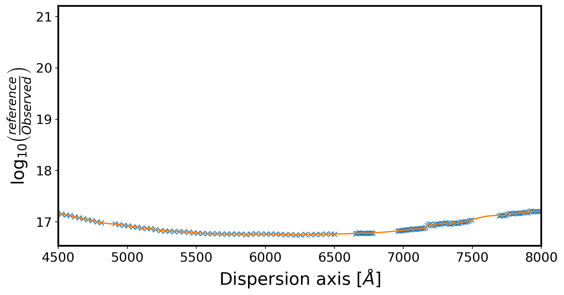
sensfunc = 10**sensfunc2
obj_cal = obj_flux*sensfunc #flux after flux calibration

fig,ax = plt.subplots(1,2,figsize=(14,4))
ax[0].plot(obj_wave,obj_flux*sensfunc)
ax[0].set_xlim(4000,8000)
ax[0].set_title('After flux calibration')
ax[0].set_ylabel(r'counts')
ax[0].set_xlabel(r'Dispersion axis $[\AA]$',fontsize=20)
ax[0].set_ylim(0,4e22)
ax[1].plot(std_wave,std_flux)
ax[1].set_xlim(4000,8000)
ax[1].set_title('Reference')
ax[1].set_ylabel(r'erg $s^{-1}cm^{-2}\AA^{-1}$ ')
ax[1].set_xlabel(r'Dispersion axis $[\AA]$',fontsize=20)
ax[1].set_ylim(0,4e22)
(0.0, 4e+22)
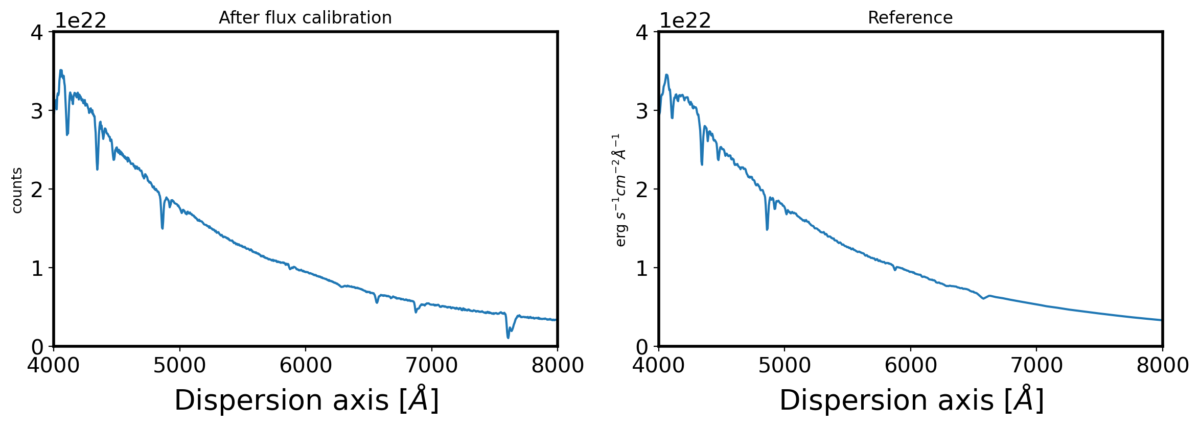
path = Objectlist[0]

tar = ascii.read(SUBPATH/('p'+path.stem+'_w_spec.csv'))
tar_wave = tar['wave']
tar_flux = tar['inten']
tar_cal = tar_flux*sensfunc #flux after flux calibration
tar_std = tar['std']*sensfunc

fig,ax = plt.subplots(1,1,figsize=(10,6))
ax.plot(tar_wave,tar_cal,c='k')
# ax.set_xlim(4000,8000)
ax.set_title('After flux calibration')
ax.set_ylabel(r'erg $s^{-1}cm^{-2}\AA^{-1}$ ')
ax.set_xlabel(r'Dispersion axis $[\AA]$',fontsize=20)
ax.set_ylim(0,1e22)

spectrum = Table([tar_wave, tar_cal, tar_std],
                names=['wave', 'flux', 'error'])
spectrum['wave'].format = "%.3f"
spectrum['flux'].format = "%.3e"
spectrum['error'].format = "%.3e"

SPEC_SAVEPATH = SUBPATH/('p'+path.stem+'_wf_spec.csv')
spectrum.write(SPEC_SAVEPATH, overwrite=True, format='csv')