PSF photometry of NGC 2210#
“Astronomers never seem to want to do anything easy.”- Peter B. Stetson (1987)
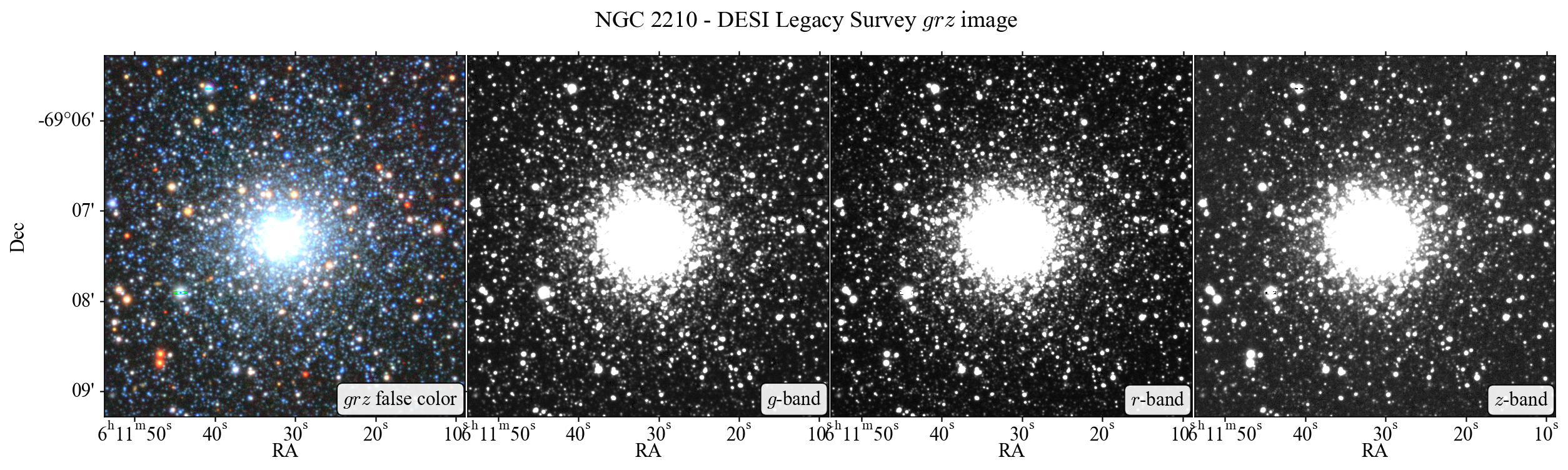
In this tutorial we will conduct some basic PSF photometry on a DESI Legacy
Survey image of the globular cluster NGC 2210. We will use the photutils.psf
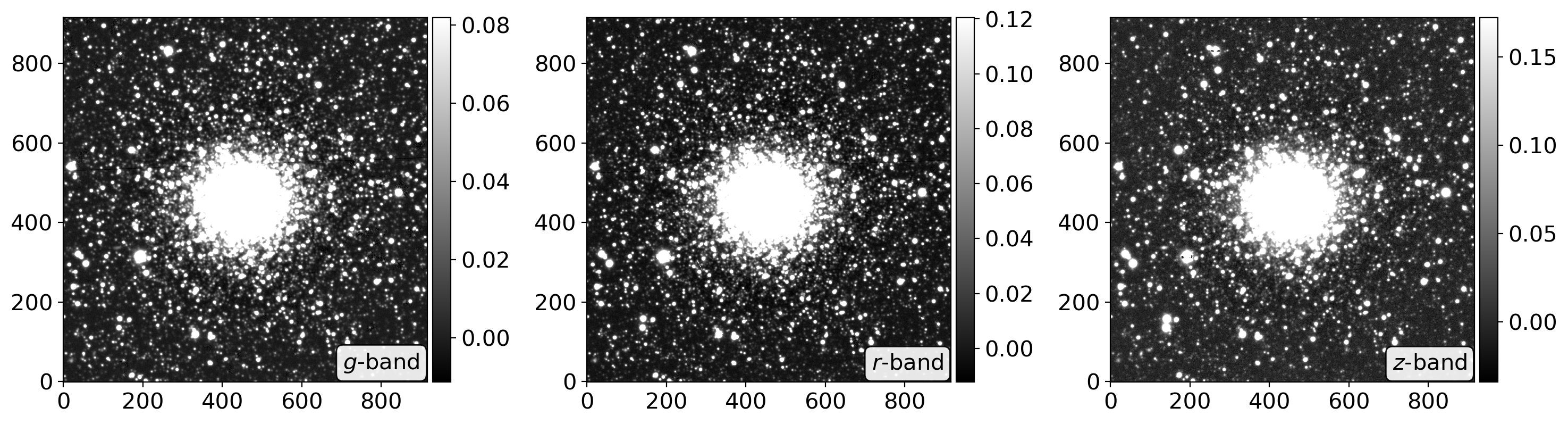
module to perform PSF photometry on the image. Below image shows each frame of
\(grz\) band and their false-color image of the NGC 2210. The aim for this
tutorial is to get \(grz\) magnitudes and colors of stars inside this field, by
PSF photometry, and to get their color-magnitude diagram for the investigation
of the properties of NGC 2210.
Reading lists#
PSF photometry
For the general understanding of the processes regarding to the astronomical photometric measurement, one can consult following references.
General Photometry
If you are not familiar with handling the astronomical data, the following tutorials may be helpful. Especially, the SNU_AOclass repository deveoloped by Yoonsoo P. Bach, which is the TA lecture note for astronomical observation class for SNU undergraduate students, will provide the most of the things you need, if you concern your lack of backgrounds.
Self-consistent general data analysis for astronomical observation
SNU AO Class Python Notes (by Yoonsoo Bach)
Useful tutorials
CCD Data Handling
CCD Data Reduction Guide (by Matthew Craig)
PSF photometry - an overview#
PSF photometry is the process of measuring the brightness of the stars by numerically fitting their light profile across the CCD image frame. For the stars isolated in the frame, the aperture photometry suffices to measure their flux and uncertainty, without any heavy computations of optimization process, and without the possibility of failure in the model to represent the stellar profile inside the frame. As Stetson (1987) mentioned, the aperture photmetry is “the most easiest and potentially most accurate method for obtaining instrumental photometry for bright, uncrowded stars, because it involves simple counting of detected photons.” (Stetson, 1987) However, for stars inside the crowded field, such as open clusters, globular clusters, and Magellanic Clouds, it is impossible to measure the brightness of blended stars by just summing their photon counts inside some apertures. Thus we have to adopt numerical fitting technique to model the brightness profile of the blended stars simultaneously, under the assumption of the linearity of the detector, and extract the total flux of a star from the model.
PSF photometry is processed in the following steps:
Subtract background light from the image
Find stars inside the frame
Define a model for stellar light profile (point spread function; PSF)
Group the blended stars which have to be simultaneously fitted
Fit the light profiles of the star groups
Examine the residual (data - model) image to decide whether or not to …
change the parameters for finding stars
reconstruct the PSF model
resize fitting window
iterate additional extraction in the residual
etc.
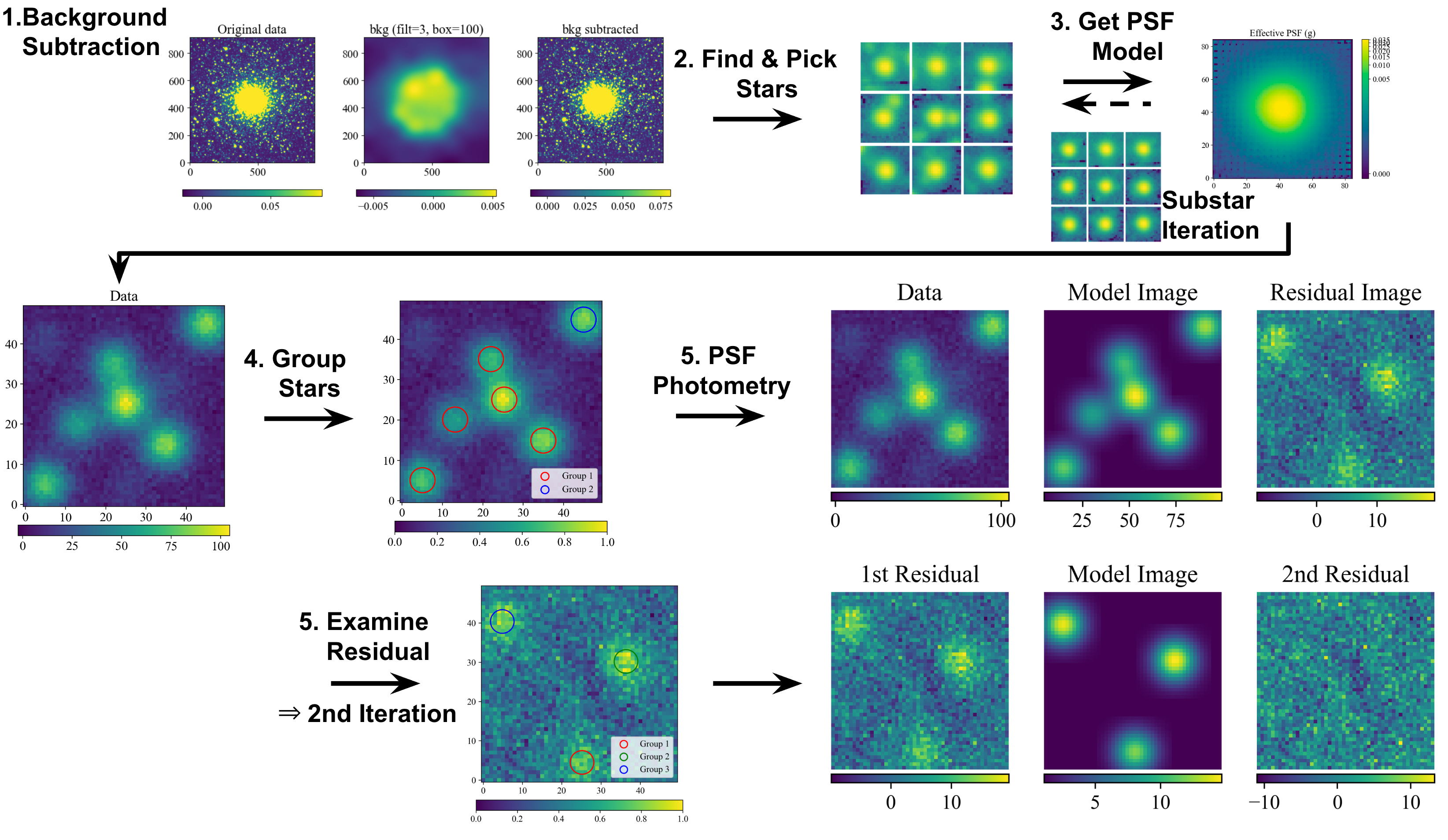
This is the outline of this tutorial regarding to the above steps.
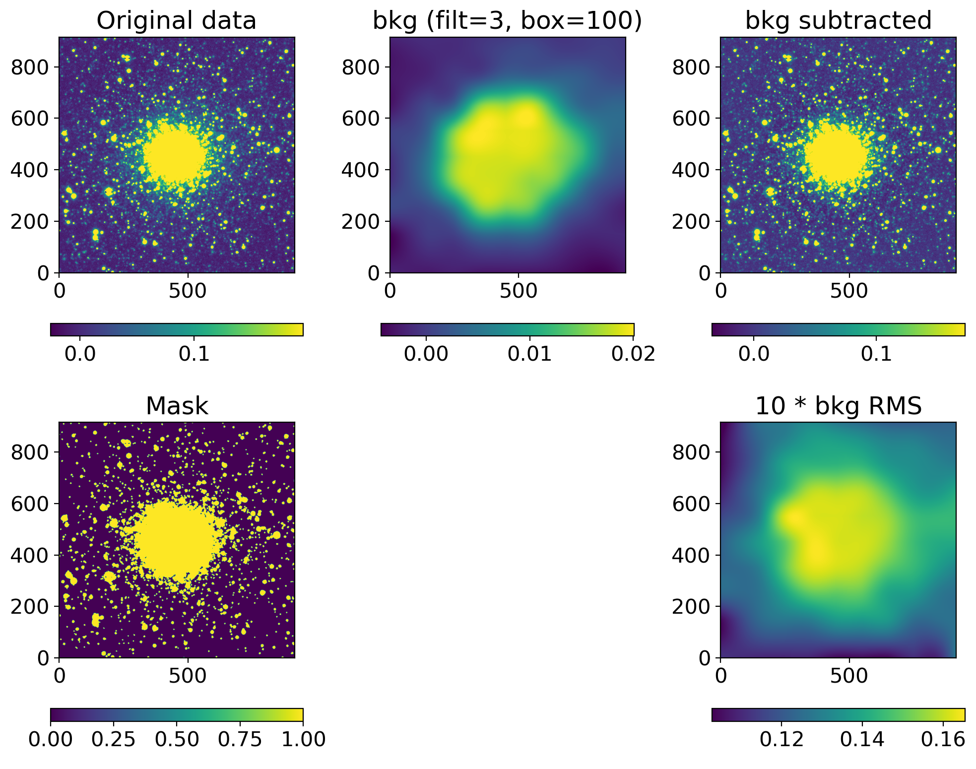
We will subtract the background of each frame using
seppackage, which is developed to replicate Source Extractor (Bertin, 1996). Here we usesep.Backgroundto subtract the background.We will first find stars with simple method
find_peaksfromphotutils.detection. This simple selection of stars will provide the stars for modeling PSF. For better modeling of PSF, one should carefully pick the bright isolated stars, but here we just adopt some simple selection criteria to pick the stars, expecting that the adjacent stars will be eventually averaged out.With the stars we picked, we derive the effective PSF (EPSF), using
EPSFBuilderfromphotutils.psf. We usephotutils.psf.extract_starsto makeEPSFStarsobject out of the table of stars we obtained byfind_peaks, then feed this object toEPSFBuilderto get the EPSF model. For better model, we can subtract the adjacent stars in the window ofEPSFStarsby fit them using the EPSF model, and rederive the EPSF from the ‘cleaned’EPSFStars.+5.
BasicPSFPhotometryfromphotutils.psfwill subtract background, find stars, group them, and fit the stellar groups to conduct PSF photometry. What we have to do is to select the background estimator (MMMBackground, which is the same with the one in DAOPHOT), star finder (DAOStarFinder; in here we input the FWHM measured from aperture photometry of stars found byfind_peak, to better performance for finding stars), fitter (LevMarLSQFitter), etc.From
BasicPSFPhotometrywe can also obtain the residual image. In this image we can examine the goodness of fit, and identify some failures of the model (Stetson 1987):images of stars which were in the frame but were not recognized by the star finder, perhaps due to having been blended with brighter companions
stars whose images contained defective pixels
images of galaxies which are almost but not quite, stellar
other similar departures from a perfect fit may be recognized and flagged
We will iterate 1-6. over all bands (\(grz\)) to get PSF photometry in different bands.
We match the stars with PSF photometry in each band. The match will be done by their positions. Here we just used the pixel coordinates, since the image we are dealing with is the cutout image from Legacy Survey so the images are aligned already. However, in more general case this is often not the case, so the match by celestial coordinates using WCS information should be better, otherwise you need to align the images first.
We will obtain colors of the matched stars and draw color-magnitude diagram of them, which are in the field of the NGC 2210.
In order to compare our PSF photometry with other results, we will use the photometry from the Legacy Survey catalog and the homoegeous photometric catalog provided by Stetson et al. (2019). To compare with the result of the latter, we will convert the DECam (the telescope used for DESI Legacy Survey) \(gr\) filter system to Johnson-Cousins \(BV\) system.
Caveat#
The DESI Legacy Survey image we adopt here is already standard-calibrated with each pixel in the unit of nanomaggy. In reality, you need to convert the instrumental flux into standard flux, with the instrumental flux of standard stars.
This tutorial is constructed with the limit of time, so this may not be complete and self-consistent, so if you have a question for this notebook ask me in person or send me an email to bahkhyeonguk@gmail.com.
%config InlineBackend.figure_format = 'retina'
No. |
Software |
Version |
|---|---|---|
0 |
Python |
3.12.2 64bit [Clang 14.0.6 ] |
1 |
IPython |
8.20.0 |
2 |
OS |
macOS 13.4.1 arm64 arm 64bit |
3 |
numpy |
1.26.4 |
4 |
matplotlib |
3.8.0 |
5 |
astropy |
5.3.4 |
6 |
photutils |
1.11.0 |
import copy
from pathlib import Path
from matplotlib import patches
from matplotlib import pyplot as plt
import numpy as np
import sys
from time import time, ctime
import warnings
from astropy.io import fits
from astropy.table import Table, hstack, vstack
from astropy.modeling.fitting import LevMarLSQFitter
from astropy.stats import sigma_clipped_stats, gaussian_fwhm_to_sigma, SigmaClip
from astropy.table import Table
from astropy.nddata import NDData, CCDData
from astropy.utils.exceptions import AstropyWarning
from astropy.visualization import simple_norm, ZScaleInterval
from photutils.aperture import CircularAperture, ApertureStats
from photutils.detection import DAOStarFinder, find_peaks
from photutils.psf import extract_stars, EPSFBuilder
from photutils.psf import DAOPhotPSFPhotometry, BasicPSFPhotometry
from photutils.psf import DAOGroup
from photutils.psf.epsf_stars import EPSFStars
from photutils.psf.utils import _extract_psf_fitting_names
from photutils.psf.utils import get_grouped_psf_model
from photutils.detection import IRAFStarFinder
from photutils.background import MMMBackground, MADStdBackgroundRMS
# from photutils.segmentation import make_source_mask
from photutils.segmentation import SegmentationImage
from photutils.segmentation import detect_threshold, detect_sources
from photutils.utils import circular_footprint
from mpl_toolkits.axes_grid1 import make_axes_locatable
import sep

sys.setrecursionlimit(10**7)
# plt.rcParams["font.family"] = 'Times New Roman'
plt.rcParams["font.size"] = 15
plt.rcParams["text.usetex"] = False
# plt.rcParams["mathtext.fontset"] = 'cm'

warnings.simplefilter('ignore', category=AstropyWarning)

WD = Path('.')
DATADIR = WD/'data'/'proj2'
OUTDIR = DATADIR/'out'

if not OUTDIR.exists():
    OUTDIR.mkdir()
1. Data Reading and Background Subtraction#
def zscale_imshow(ax, img, vmin=None, vmax=None, **kwargs):
if vmin==None or vmax==None:
interval = ZScaleInterval()
_vmin, _vmax = interval.get_limits(img)
if vmin==None:
vmin = _vmin
if vmax==None:
vmax = _vmax
im = ax.imshow(img, vmin=vmin, vmax=vmax, origin='lower', **kwargs)
return im
def read_sci_data(fpath, show=True, newbyteorder=False, bkgsubtract=False):
ccd_raw = CCDData.read(fpath, unit='nmgy') # be careful about the unit!
ccd = CCDData.read(fpath, unit='nmgy')
data = ccd.data
data_mean, data_med, data_std = sigma_clipped_stats(data, sigma=2.)
ccd.mask = data < data_mean - 3*data_std
ccd.data[ccd.mask] = data_med
ccd.data -= data_med
ccd.mask = (ccd.mask) & (data > 10.)
if newbyteorder:
ccd.data = ccd.data.byteswap().newbyteorder()
n = len(ccd.data)
if bkgsubtract:
bkgsubs = []
for i in range(n):
bkgsub = background_substraction(ccd.data[i])
bkgsubs.append(bkgsub)
ccd.data = np.array(bkgsubs)
if show:
fig, axes = plt.subplots(1, n, figsize=(5*n, 5))
for i in range(n):
im = zscale_imshow(axes[i], ccd.data[i], cmap='gray')
divider = make_axes_locatable(axes[i])
cax = divider.append_axes('right', size='5%', pad=0.05)
fig.colorbar(im, cax=cax, orientation='vertical')
band = ccd.header[f'BAND{i}']
axes[i].text(0.98, 0.02, f'${band}$-band',
transform=axes[i].transAxes,
va='bottom', ha='right', c='k',
bbox=dict(boxstyle='round', facecolor='w', alpha=0.9))
plt.tight_layout()
return ccd, ccd_raw
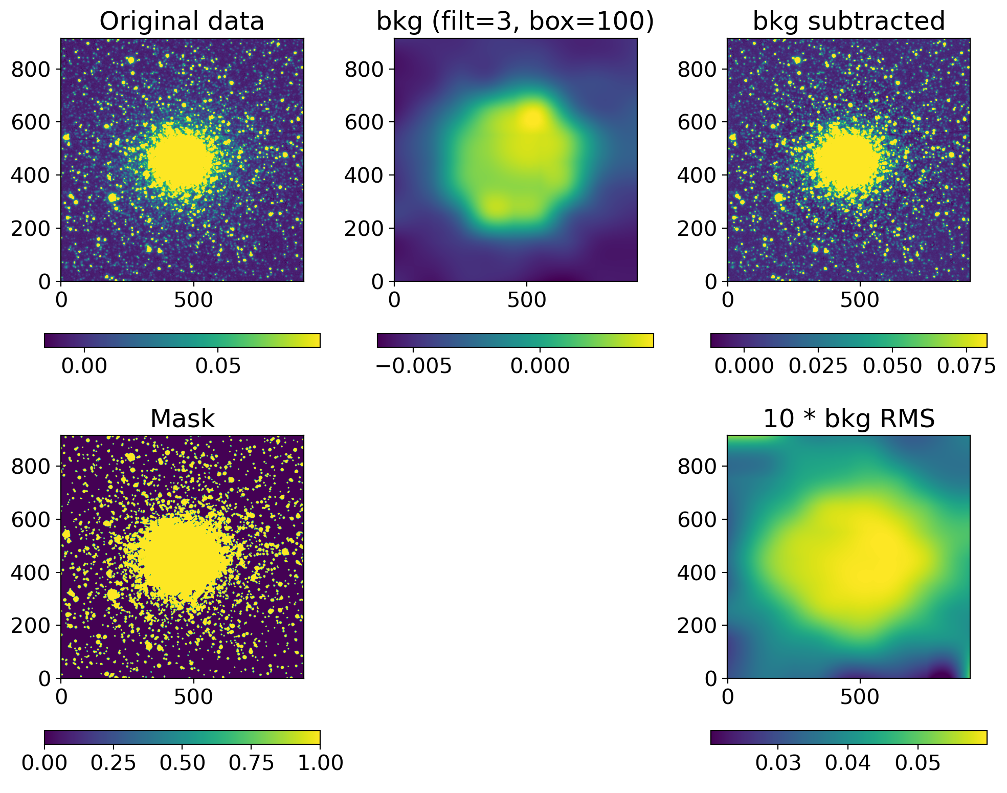
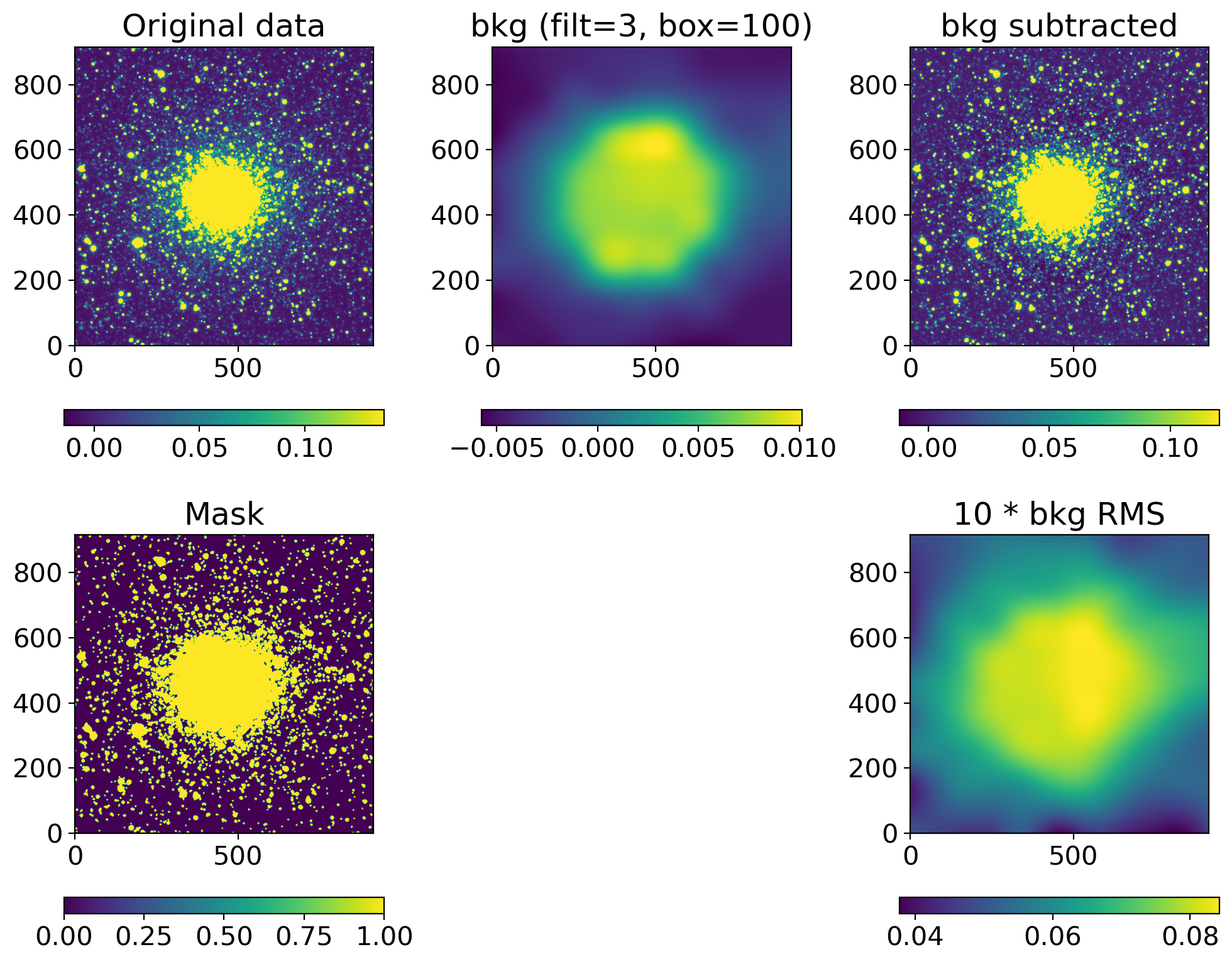
def background_substraction(img, box=100, filt=3, show=True):
sigma_clip = SigmaClip(sigma=3.0, maxiters=10)
threshold = detect_threshold(img, nsigma=3.0, sigma_clip=sigma_clip)
segment_img = detect_sources(img, threshold, npixels=10)
footprint = circular_footprint(radius=1)
mask = segment_img.make_source_mask(footprint=footprint)
# mask = SegmentationImage.make_source_mask(img, nsigma=2, npixels=1, dilate_size=3)
bkg_sep = sep.Background(img.byteswap().newbyteorder(),
mask=mask, bw=box, bh=box, fw=filt, fh=filt)
bkgsub_sep = img - bkg_sep.back()
if show:
fig, axs = plt.subplots(2, 3, figsize=(10, 8))
axs[1, 1].axis("off")
data2plot = [
dict(ax=axs[0, 0], arr=img, title="Original data"),
dict(ax=axs[0, 1], arr=bkg_sep.back(), title=f"bkg (filt={filt:d}, box={box:d})"),
dict(ax=axs[0, 2], arr=bkgsub_sep, title="bkg subtracted"),
dict(ax=axs[1, 0], arr=mask, title="Mask"),
# dict(ax=axs[1, 1], arr=bkg_sep.background_mesh, title="bkg mesh"),
dict(ax=axs[1, 2], arr=10*bkg_sep.rms(), title="10 * bkg RMS")
]
for dd in data2plot:
im = zscale_imshow(dd['ax'], dd['arr'])
cb = fig.colorbar(im, ax=dd['ax'], orientation='horizontal')
# cb.ax.set_xticklabels([f'{x:.3f}' for x in cb.get_ticks()])#, rotation=45)
dd['ax'].set_title(dd['title'])
plt.tight_layout()
return bkgsub_sep
ccd, ccd_raw = read_sci_data(DATADIR/'NGC2210.grz.fits', bkgsubtract=True)
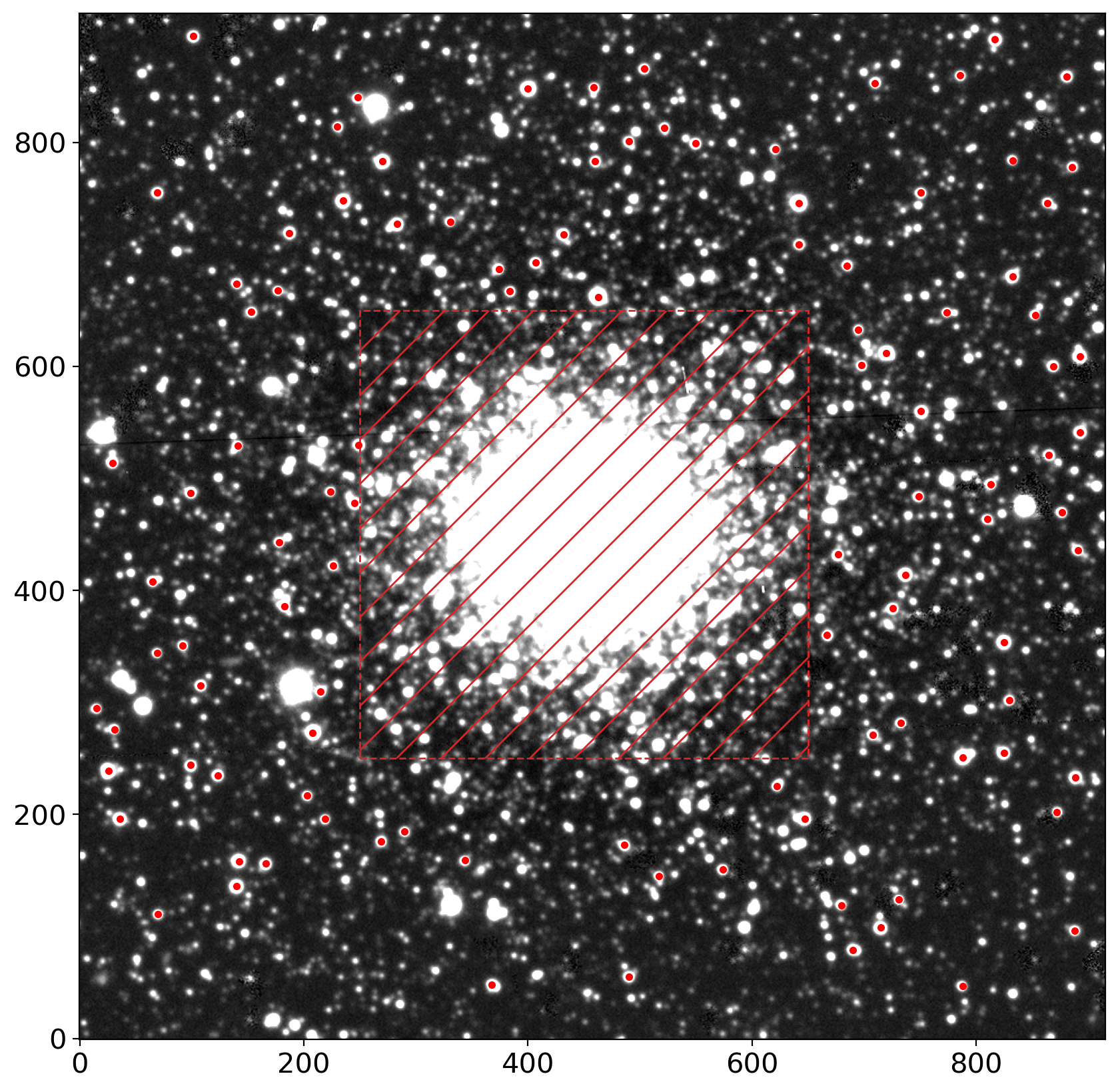
2. Selection of Stars for the PSF Estimation#
bands = ['g', 'r', 'z']
i = 0
band = bands[i]
data = ccd.data[i]
mask = ccd.mask[i]
bkgrms = MADStdBackgroundRMS()
std = bkgrms(data)
thres = 3*std
find_mask = np.zeros_like(data, dtype=bool)
# find_mask[250:650, 250:650] = True
# ll, hh = 0, 200
ll, hh = 250, 650
find_mask[ll:hh, ll:hh] = True
peaks_tbl = find_peaks(data, threshold=thres, mask=find_mask)
peaks_tbl['peak_value'].info.format = '%.8g'
print('number of peaks:', len(peaks_tbl))
peaks_tbl[:5].show_in_notebook()
# select stars within the cutout of specified size, which must be odd
size = 21 # typically ~4*FWHM. user should consider the PSF size for selecting this value
hsize = (size - 1) / 2
x = peaks_tbl['x_peak']
y = peaks_tbl['y_peak']
bound = ((x > hsize) & (x < (data.shape[1] -1 - hsize)) &
(y > hsize) & (y < (data.shape[0] -1 - hsize)))
bright = (peaks_tbl['peak_value'] > 0.5) & (peaks_tbl['peak_value'] < 10.)
bbmask = (bound & bright)
bx, by = x[bbmask], y[bbmask]
isolated = [False if np.count_nonzero(np.sqrt((bx-xi)**2+(by-yi)**2)<size) > 1
else True for xi, yi in zip(bx, by)]
mask_stars = isolated
# mask_stars = np.ones_like(bx, dtype=bool)
stars_tbl = Table()
stars_tbl['x'] = bx[mask_stars]
stars_tbl['y'] = by[mask_stars]
print('number of stars picked:', len(stars_tbl))
stars_tbl[:5].show_in_notebook()
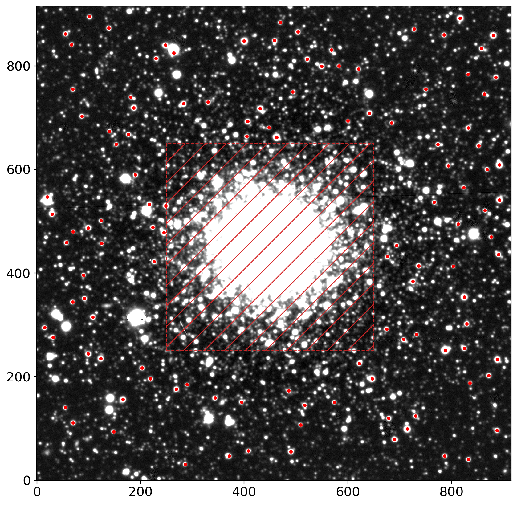
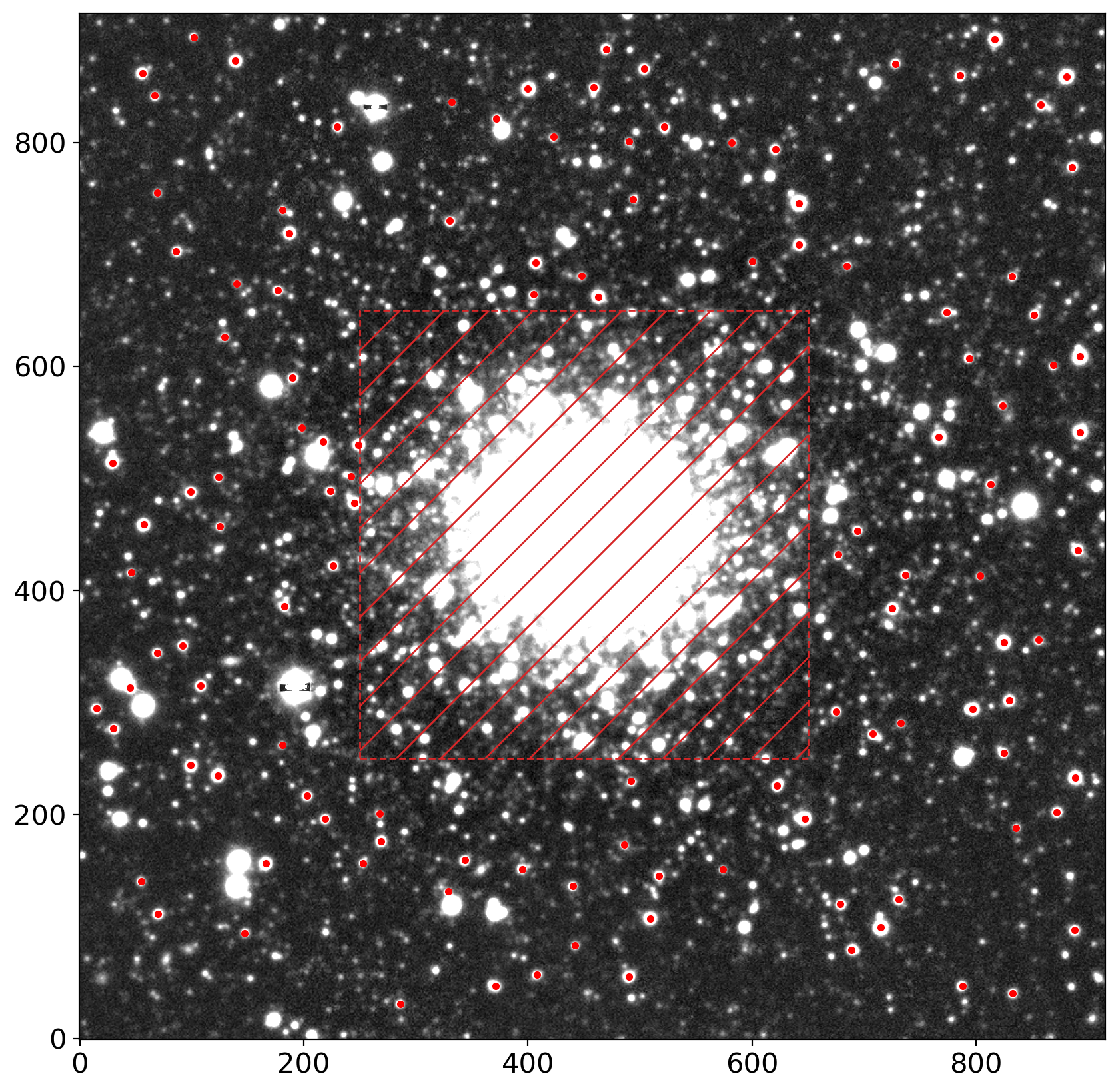
nddata = NDData(data=data, mask=ccd.mask[i])
# plot the locations of our selected stars
fig, ax = plt.subplots(1, 1, figsize=(10, 10))
im = zscale_imshow(ax, data, cmap='gray')
ax.plot(stars_tbl['x'], stars_tbl['y'], '.r')
rect = patches.Rectangle((ll,ll), hh-ll, hh-ll, ec='tab:red', ls='--',
hatch='/', fc='none', lw=1)
ax.add_patch(rect)
number of peaks: 3781
number of stars picked: 107
<matplotlib.patches.Rectangle at 0x176215400>
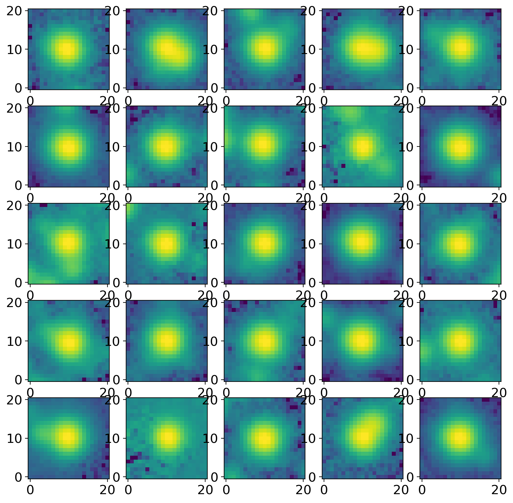
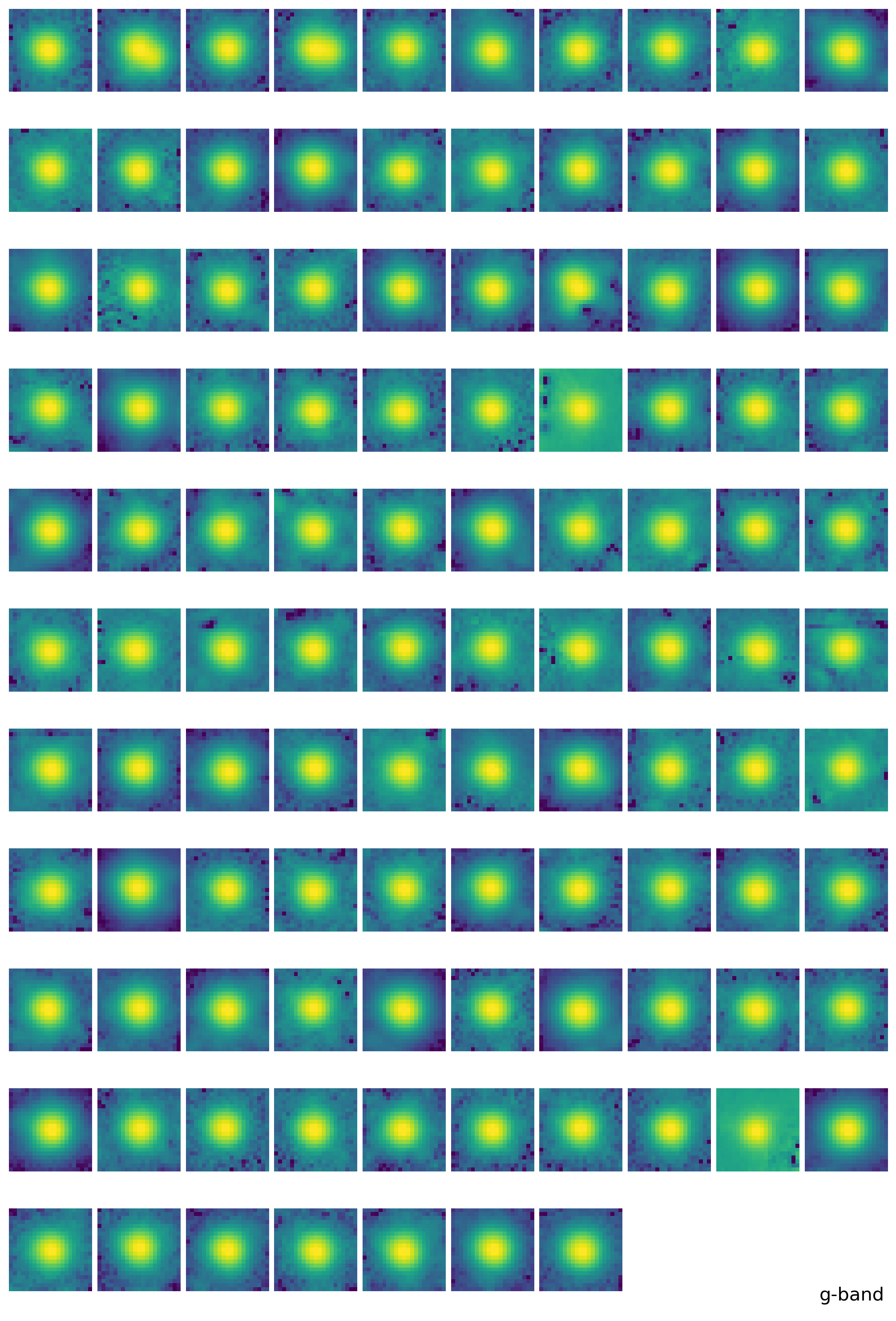
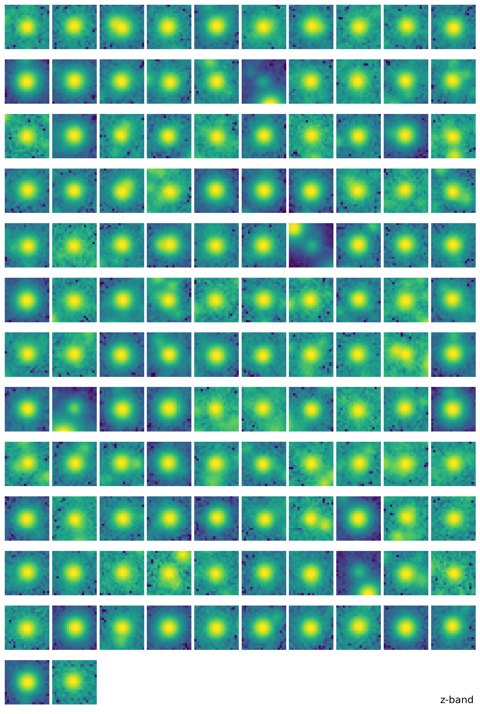
# extract cutouts of our selected stars
stars = extract_stars(nddata, stars_tbl, size=size)

# plot cutouts
nrows = 5
ncols = 5
fig, ax = plt.subplots(nrows=nrows, ncols=ncols, figsize=(10, 10),
                       squeeze=True)
ax = ax.ravel()
for i in range(nrows * ncols):
    norm = simple_norm(stars[i], 'log', percent=99.0)
    ax[i].imshow(stars[i], norm=norm, origin='lower', cmap='viridis')

# derive fwhm from aperture statistics
cap = CircularAperture(stars.center_flat, size/5.)
apstat = ApertureStats(data, cap)

fwhm_mean, fwhm_med, fwhm_std = sigma_clipped_stats(apstat.fwhm.value,
                                                    sigma=3.0)
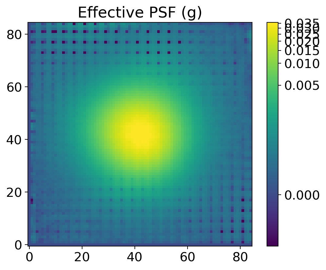
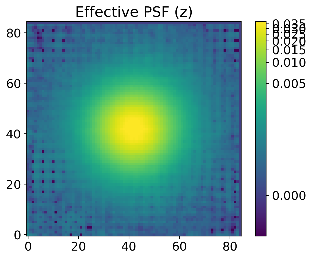
3. Derive Effective PSF#
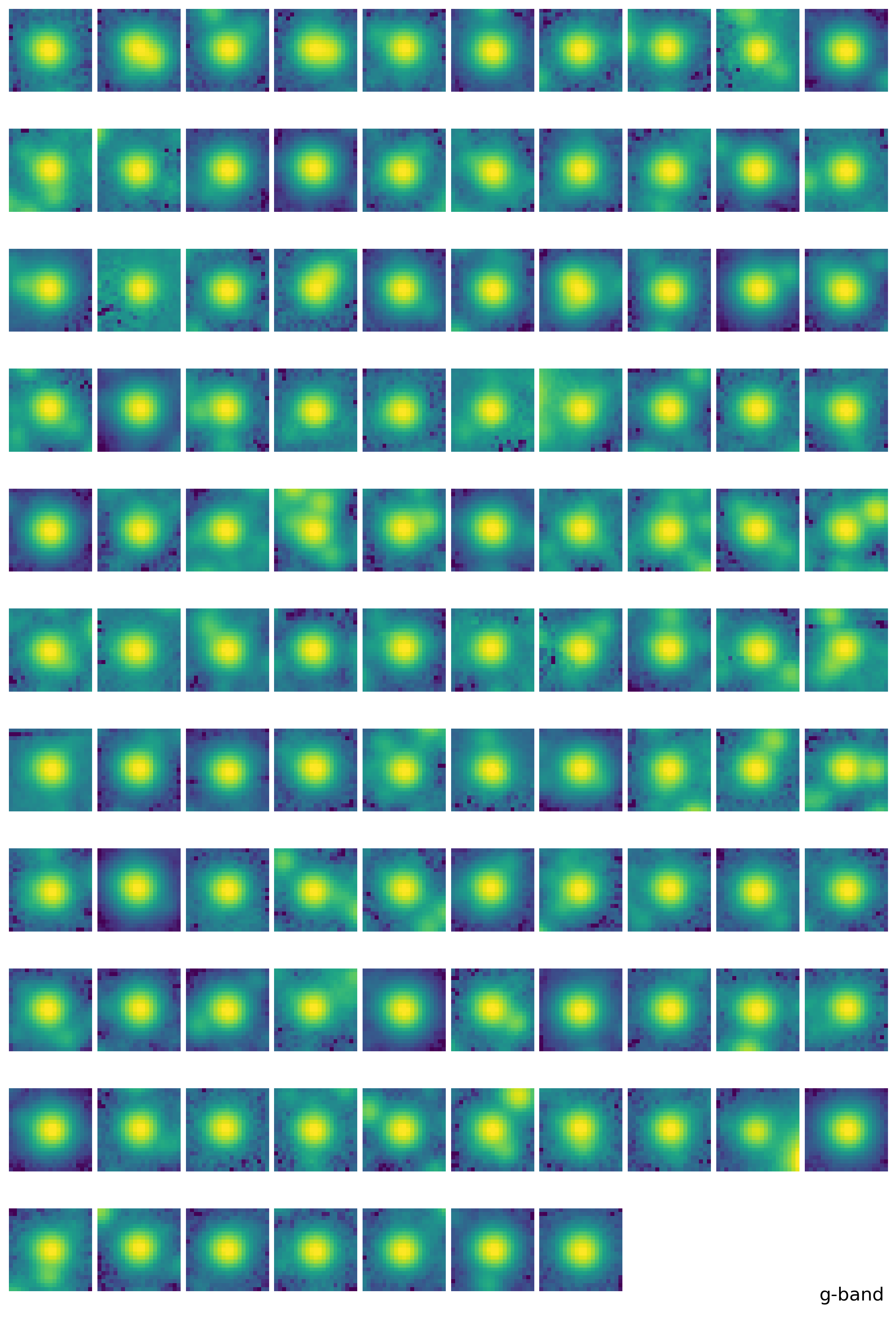
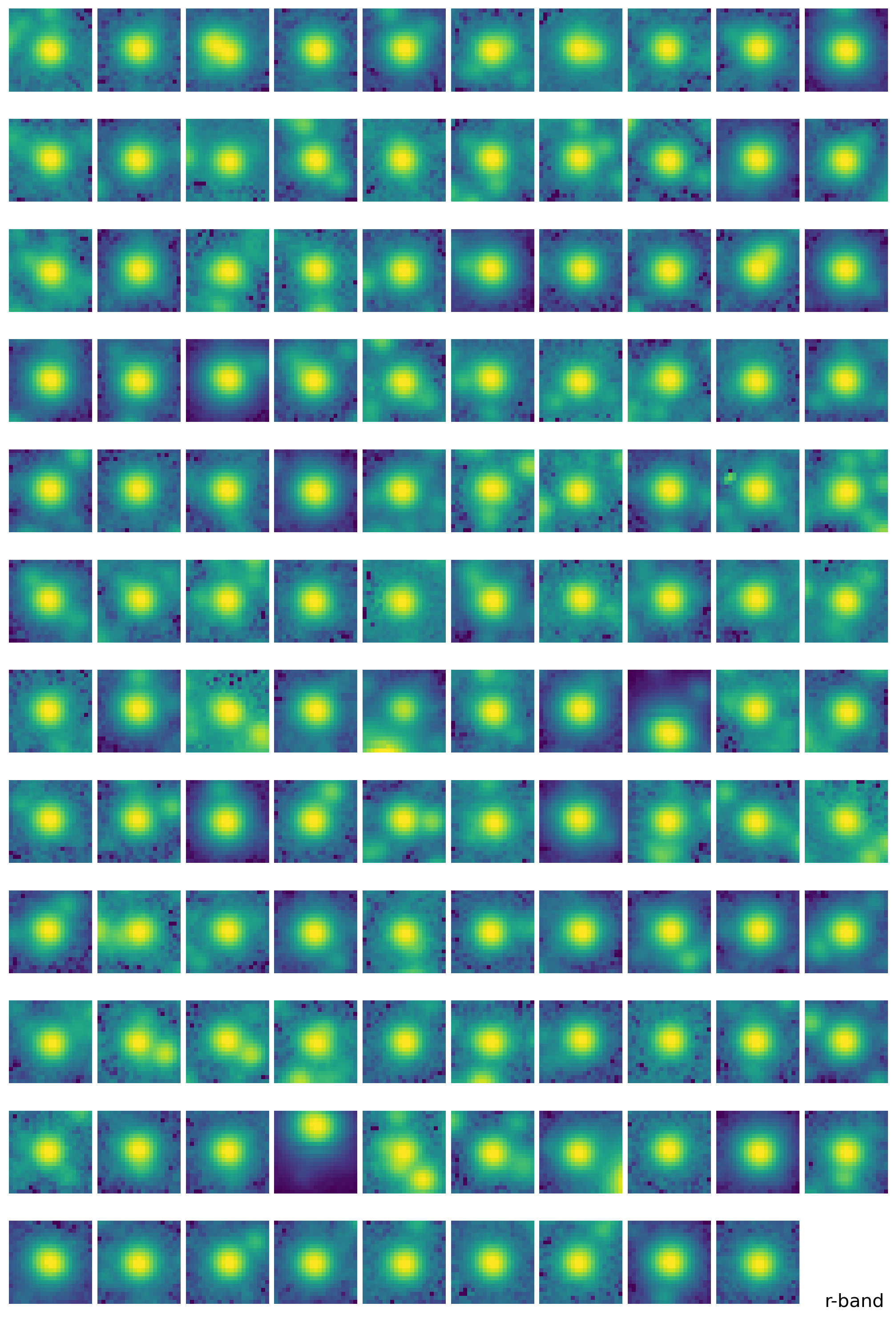
def get_epsf(stars, band,
oversampling=4, maxiters=10, smoothing_kernel='quadratic',
show=True, ncols=None, figsize=(10, 15)):
if show:
if ncols == None:
n, m = figsize
ncols = n * np.round(np.sqrt(len(stars)/n/m)).astype(int)
nrows = int(np.ceil(len(stars)/ncols))
fig, axs = plt.subplots(nrows=nrows, ncols=ncols, figsize=figsize,
squeeze=True)
axs = axs.ravel()
for ax in axs:
ax.axis('off')
for i in range(len(stars)):
norm = simple_norm(stars[i], 'log', percent=99.)
axs[i].imshow(stars[i], norm=norm, origin='lower', cmap='viridis')
fig.text(0.99,0.01,f'{band}-band',
ha='right', va='bottom', fontsize=15)
# fig.suptitle(f'Picked stars to model PSF ({band})')
plt.tight_layout(pad=0.3)
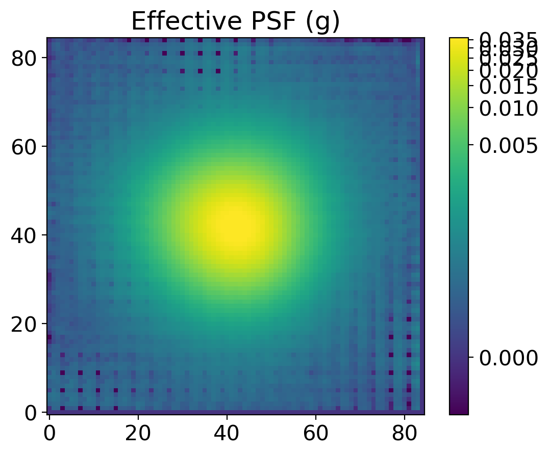
epsf_builder = EPSFBuilder(oversampling=oversampling, maxiters=maxiters,
progress_bar=False,
smoothing_kernel=smoothing_kernel)
epsf, fitted_stars = epsf_builder(stars)
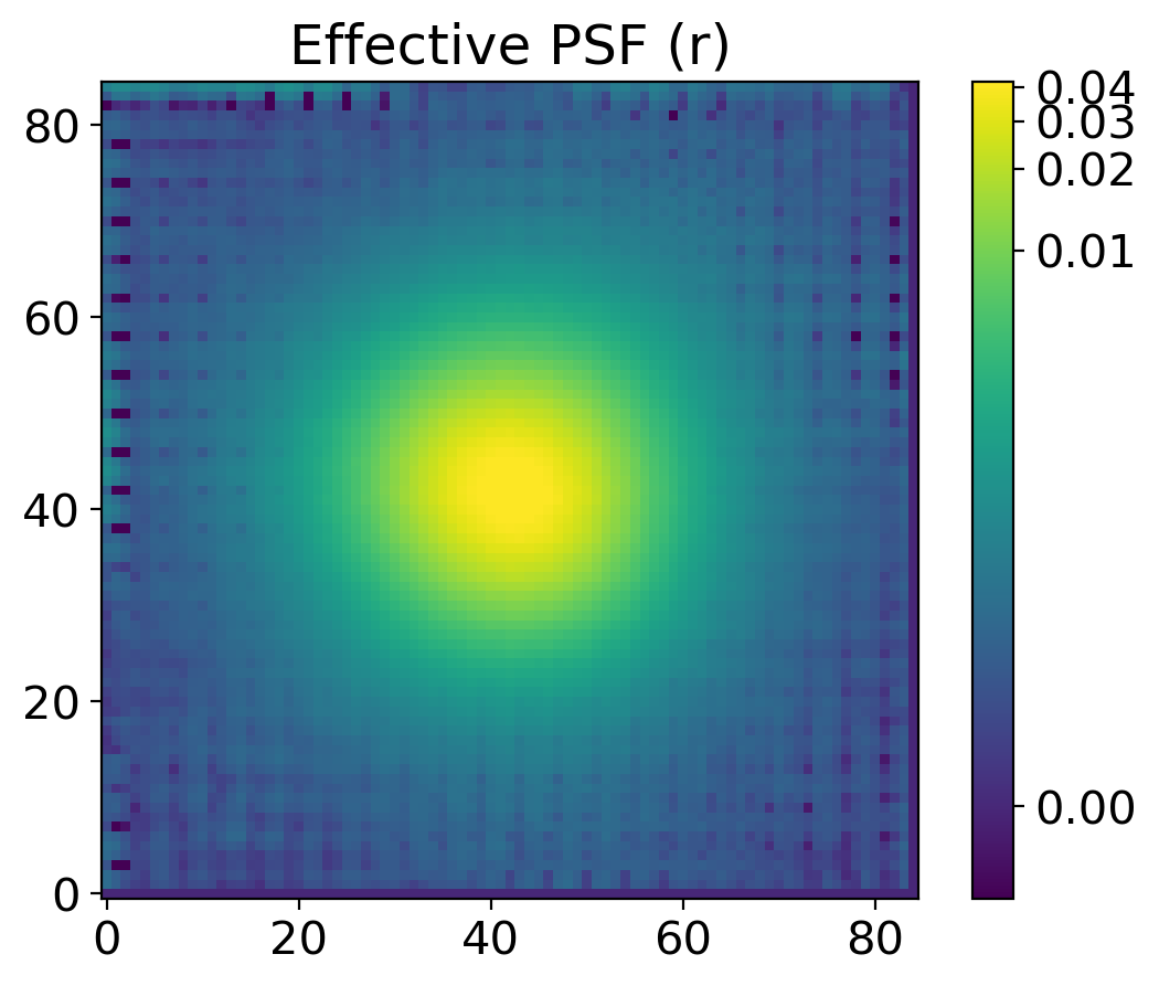
if show:
plt.figure()
norm = simple_norm(epsf.data, 'log', percent=99.)
plt.imshow(epsf.data, norm=norm, origin='lower', cmap='viridis')
plt.title(f'Effective PSF ({band})')
plt.colorbar()
return epsf
epsf0 = get_epsf(stars, band)
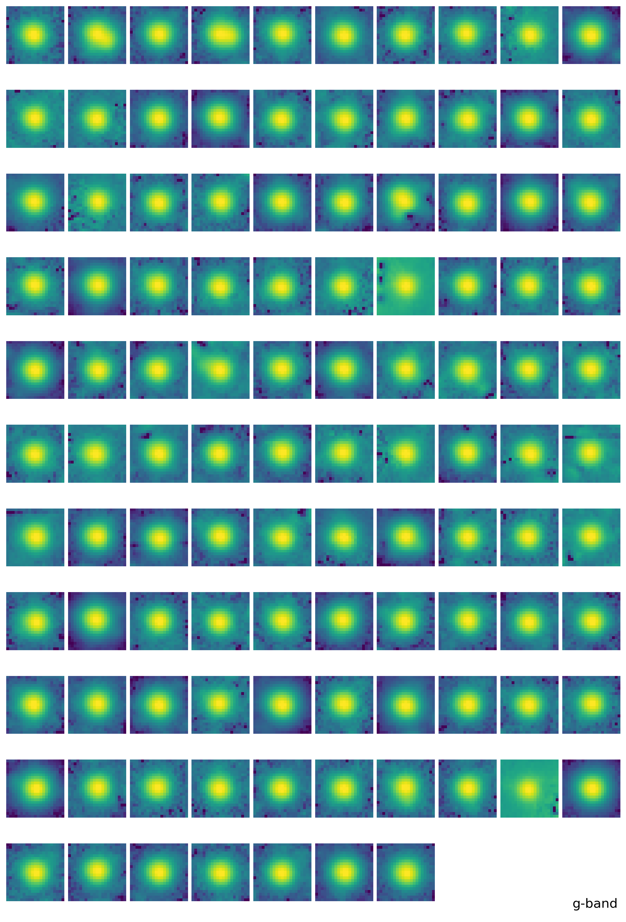
SUBSTAR - subtract adjacent stars and reconstruct EPSF#
# substar procedure
# subtract adjacent star profiles using the epsf model we obtained.

def get_substars(stars, psf_model, thres, fwhm, band, peakmax=None,
            show=True, ncols=10, figsize=(10, 15)):
    substars_list = []
    for star in stars:
        finder = DAOStarFinder(threshold=thres, fwhm=fwhm,
                               roundhi=5.0, roundlo=-5.0,
                               sharplo=0.0, sharphi=2.0, peakmax=peakmax)
        found = finder(star.data)
        found.rename_columns(['xcentroid', 'ycentroid', 'flux'],
                             ['x_0', 'y_0', 'flux_0'])
        if len(found) > 1:
            fitter = LevMarLSQFitter()
            y, x = np.indices(star.shape)
            xname, yname, fluxname = _extract_psf_fitting_names(psf_model)
            pars_to_set = {'x_0': xname, 'y_0': yname, 'flux_0': fluxname}
            group_psf = get_grouped_psf_model(psf_model, found, pars_to_set)
            fit_model = fitter(group_psf, x, y, star.data)

            if hasattr(star, 'cutout_center'):
                xc, yc = star.cutout_center
            elif hasattr(star, 'cutout_center_flat'):
                xc, yc = star.cutout_center_flat[0]
            else:
                raise AttributeError
            idx = np.argmin((found['x_0']-xc)**2+(found['y_0']-yc)**2) # crude
            cent_model = fit_model[idx]

            substar_data = star.data - fit_model(x, y) + cent_model(x, y)
            mask = np.ones_like(substar_data, dtype=bool)
            hsize = substar_data.shape[0]//2
            psize = int(fwhm)*2
            mask[hsize-psize:hsize+psize, hsize-psize:hsize+psize] = False
            _, med, sig = sigma_clipped_stats(substar_data[mask], sigma=2.0)
            # substar_data[substar_data < med-2*sig] = med
            substar_data = substar_data - med

            substar = copy.deepcopy(star)
            substar._data = substar_data
        else:
            substar = star

        substars_list.append(substar)

    substars = EPSFStars(substars_list)
    return substars
substars = get_substars(stars, epsf0, 2*std, fwhm_mean, band)
epsf1 = get_epsf(substars, band)
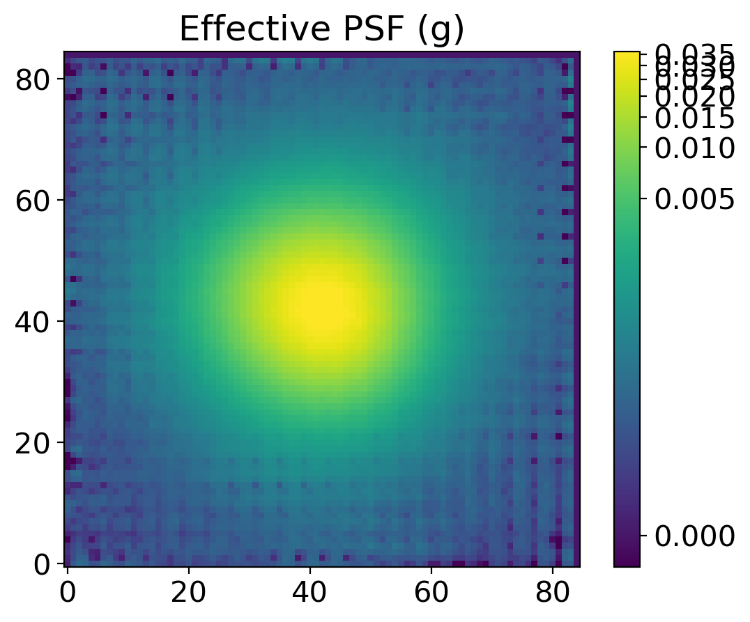
substars2 = get_substars(substars, epsf0, 1*std, fwhm_mean, band)
epsf2 = get_epsf(substars2, band)
4. PSF Photometry with the EPSF#
def get_psfphot(data, mask, psf_model, fwhm, psf_size, sigma_thres=3.,
                peakmax=None):
    # set up the photometry object
    bkgrms = MADStdBackgroundRMS()
    std = bkgrms(data) # background rms

    threshold = sigma_thres * std # threshold for star finding
    crit_separation = 2.0 * fwhm # critical separation for star grouping

    daogroup = DAOGroup(crit_separation) # grouping algorithm
    mmm_bkg = MMMBackground() # bkg estimator
    fitter = LevMarLSQFitter() # psf model fitter

    fsize = int(np.ceil(psf_size))
    fitshape = fsize if fsize%2 == 1 else fsize +1 # size of the fitting region

    # find stars for the initial guess
    daofind = DAOStarFinder(threshold=threshold,
                            fwhm=fwhm, #sigma_psf * gaussian_sigma_to_fwhm,
                            roundhi=5.0, roundlo=-5.0,
                            sharplo=0.0, sharphi=2.0, peakmax=peakmax)
    stars = daofind(data, mask=mask)

    # define the photometry object
    photometry = BasicPSFPhotometry(finder=daofind,
                                    group_maker=daogroup,
                                    bkg_estimator=mmm_bkg,
                                    psf_model=psf_model,
                                    fitter=fitter,
                                    aperture_radius=1.5*fwhm,
                                    # niters=1,
                                    fitshape=fitshape)

    # rename columns to match the names in the table
    stars.rename_columns(['xcentroid','ycentroid','flux'],
                         ['x_0', 'y_0', 'flux_0'])

    start = time() # to record the time
    print('start time -', ctime(start))

    # run the photometry
    result_tab = photometry.do_photometry(image=data, mask=mask,
                                          init_guesses=stars,
                                          progress_bar=True)
    residual_image = photometry.get_residual_image()

    finish = time()
    print('finish time -', ctime(finish))
    print(f'elapsed time - {(finish-start)/60:.2f} min')

    # discard stars outside the image
    shape = data.shape
    result_tab = discard_stars_outside(shape, result_tab)

    return result_tab, photometry


def discard_stars_outside(shape, result_tab):
    ny, nx = shape
    xin = np.logical_and(result_tab['x_fit'] > 0 , result_tab['x_fit'] < nx-1)
    yin = np.logical_and(result_tab['y_fit'] > 0 , result_tab['y_fit'] < ny-1)
    isin = np.logical_and(xin, yin)
    return result_tab[isin]
# set fwhm, psf_model, psf_size, sigma_thres, peakmax
fwhm = fwhm_med # median fwhm of selected stars
sigma_psf = fwhm * gaussian_fwhm_to_sigma # sigma of psf
psf_model = epsf0 # epsf model - just using the epsf without iteration
psf_size = fwhm * 4 # size of psf model to fit
sigma_thres = 5.0 # threshold for star detection
peakmax = 10.0 # maximum peak value for the detection (prevent saturated stars)

# get photometry by BasicPSFPhotometry
res = get_psfphot(data, mask, psf_model, fwhm, psf_size,
                  sigma_thres=sigma_thres, peakmax=peakmax)

result_tab, photometry = res # extract result table and photometry object
residual_image = photometry.get_residual_image() # residual_image = data-model

# save results
hdu = fits.PrimaryHDU(residual_image)
hdu.writeto(OUTDIR/f'res_{band}_{sigma_thres:.1f}.fits', overwrite=True)
result_tab.write(OUTDIR/f'result_tab_{band}_{sigma_thres:.1f}.csv',
                 format='csv', overwrite=True)
start time - Tue Apr 2 21:20:56 2024
finish time - Tue Apr  2 21:21:32 2024
elapsed time - 0.60 min
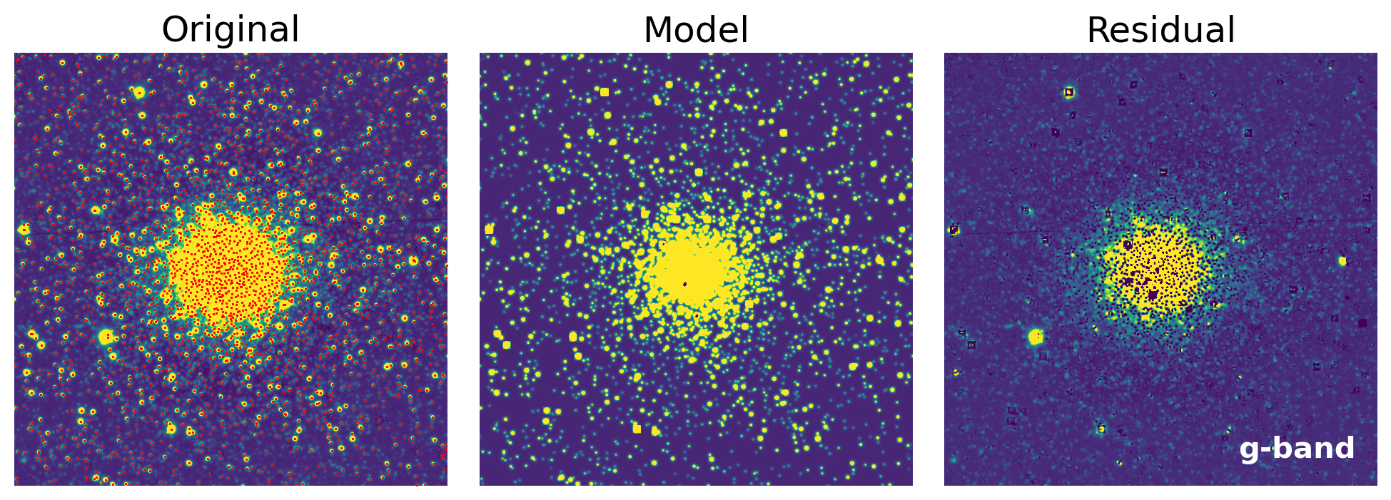
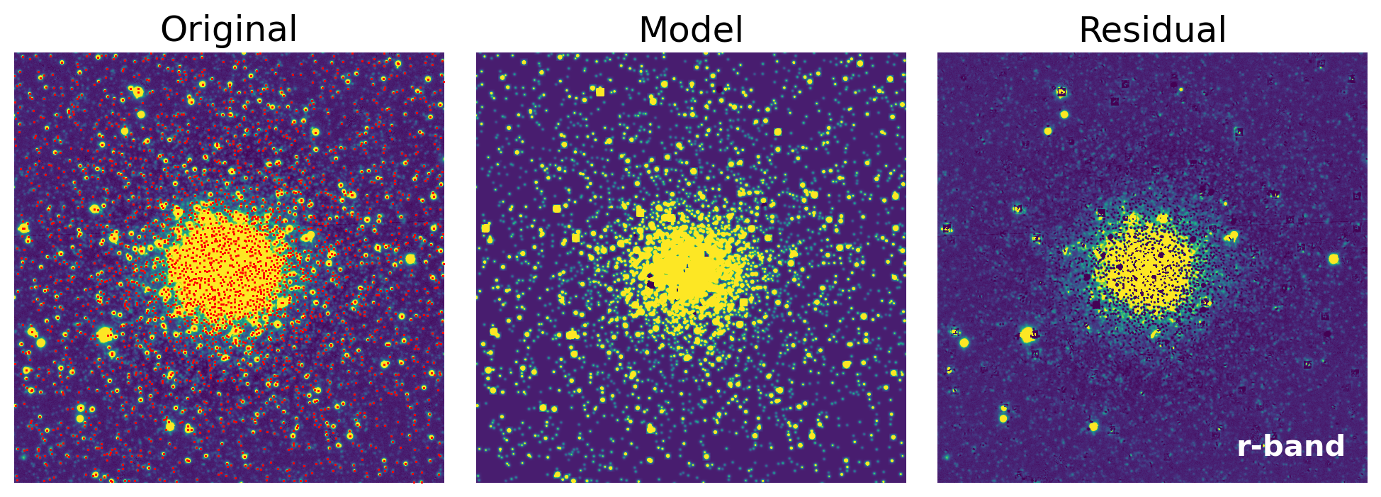
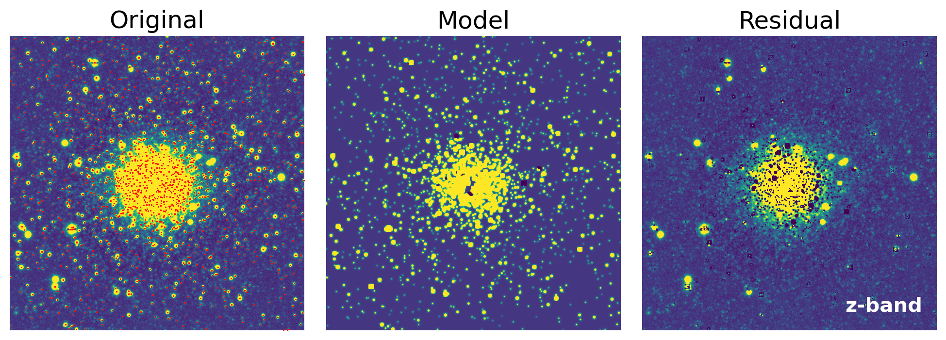
def show_psfphot_result(data, band, result_tab, residual_image):
    fig, axs = plt.subplots(1, 3, figsize=(10, 4))
    interval = ZScaleInterval()
    vmin, vmax = interval.get_limits(data)

    zscale_imshow(axs[0], data, vmin, vmax)
    zscale_imshow(axs[1], data - residual_image, vmin, vmax)
    zscale_imshow(axs[2], residual_image, vmin, vmax)
    axs[0].plot(result_tab['x_fit'], result_tab['y_fit'], marker='+', c='r',
                ms=1, ls='None')
    axs[2].text(0.95, 0.05, f'{band}-band', ha='right', va='bottom',
                   c='w', fontweight='bold', transform=axs[2].transAxes)
    axs[0].set_title('Original')
    axs[1].set_title('Model')
    axs[2].set_title('Residual')
    axs = axs.ravel()
    for ax in axs:
        ax.axis('off')

    plt.tight_layout()

    return fig
# plot results - data, model, residual
fig = show_psfphot_result(data, band, result_tab, residual_image)
5. Iterations Over All Bands#
# Let's do the same for all bands
bands = ['g', 'r', 'z']
for i in range(1, len(bands)):
    band = bands[i]
    data = ccd.data[i]
    mask = ccd.mask[i]

    print(f'### Band: {band}')
    bkgrms = MADStdBackgroundRMS()
    std = bkgrms(data)
    thres = 3*std

    find_mask = np.zeros_like(data, dtype=bool)
    ll, hh = 250, 650
    find_mask[ll:hh, ll:hh] = True
    peaks_tbl = find_peaks(data, threshold=thres, mask=find_mask)
    peaks_tbl['peak_value'].info.format = '%.8g'

    # select stars within the cutout of specified size
    size = 21
    hsize = (size - 1) / 2
    x = peaks_tbl['x_peak']
    y = peaks_tbl['y_peak']
    bound = ((x > hsize) & (x < (data.shape[1] -1 - hsize)) &
            (y > hsize) & (y < (data.shape[0] -1 - hsize)))
    bright = (peaks_tbl['peak_value'] > 0.5) & (peaks_tbl['peak_value'] < 10.)

    bbmask = (bound & bright)
    bx, by = x[bbmask], y[bbmask]

    isolated = [False if np.count_nonzero(np.sqrt((bx-xi)**2+(by-yi)**2)<size) > 1
                else True for xi, yi in zip(bx, by)]

    mask_stars = isolated
    # mask_stars = np.ones_like(bx, dtype=bool)

    stars_tbl = Table()
    stars_tbl['x'] = bx[mask_stars]
    stars_tbl['y'] = by[mask_stars]

    # print(stars_tbl)

    nddata = NDData(data=data, mask=ccd.mask[i])

    # plot the locations of our selected stars
    fig, ax = plt.subplots(1, 1, figsize=(10, 10))
    im = zscale_imshow(ax, data, cmap='gray')
    ax.plot(stars_tbl['x'], stars_tbl['y'], '.r')
    rect = patches.Rectangle((ll,ll), hh-ll, hh-ll, ec='tab:red', ls='--',
                            hatch='/', fc='none', lw=1)
    ax.add_patch(rect)

    # extract cutouts of our selected stars
    stars = extract_stars(nddata, stars_tbl, size=size)

    # derive fwhm from aperture statistics
    cap = CircularAperture(stars.center_flat, size/5.)
    apstat = ApertureStats(data, cap)

    fwhm_mean, fwhm_med, fwhm_std = sigma_clipped_stats(apstat.fwhm.value,
                                                        sigma=3.0)

    epsf0 = get_epsf(stars, band)
#     substars = get_substars(stars, epsf0, 2*std, fwhm_mean, band)
#     epsf1 = get_epsf(substars, band)
#     substars2 = get_substars(substars, epsf0, 1*std, fwhm_mean, band)
#     epsf2 = get_epsf(substars2, band)

    fwhm = fwhm_med
    sigma_psf = fwhm * gaussian_fwhm_to_sigma
    psf_model = epsf0
    psf_size = fwhm * 4
    sigma_thres = 5.
    peakmax=10.0

    res = get_psfphot(data, mask, psf_model, fwhm, psf_size,
                    sigma_thres=sigma_thres, peakmax=peakmax)

    result_tab, photometry = res
    residual_image = photometry.get_residual_image()

    hdu = fits.PrimaryHDU(residual_image)
    hdu.writeto(OUTDIR/f'res_{band}_{sigma_thres:.1f}.fits', overwrite=True)
    result_tab.write(OUTDIR/f'result_tab_{band}_{sigma_thres:.1f}.csv', format='csv', overwrite=True)

    show_psfphot_result(data, band, result_tab, residual_image)
### Band: r
start time - Tue Apr  2 21:21:39 2024
finish time - Tue Apr  2 21:22:18 2024
elapsed time - 0.67 min
### Band: z
start time - Tue Apr  2 21:22:24 2024
finish time - Tue Apr  2 21:22:43 2024
elapsed time - 0.32 min
# now let's bring the results together to match the stars from each band

sigma_thres = 5.0 # threshold for detection
tbls = []
for band in bands:
    tbls.append(Table.read(OUTDIR/f'result_tab_{band}_{sigma_thres:.1f}.csv'))

gtbl, rtbl, ztbl = tbls # extract the tables for each band

gtbl[:5].show_in_notebook()
# gtbl.show_in_notebook(display_length=10)
| idx | id | x_0 | y_0 | sharpness | roundness1 | roundness2 | npix | sky | peak | flux_0 | mag | group_id | x_fit | y_fit | flux_fit | flux_unc | x_0_unc | y_0_unc |
|---|---|---|---|---|---|---|---|---|---|---|---|---|---|---|---|---|---|---|
| 0 | 5 | 851.4578319217419 | 1.2431922857817184 | 0.3622949160971678 | -0.43358245491981506 | -0.6376099061779756 | 25 | 0.0 | 0.05964961275458336 | 2.6161646842956543 | -1.0441626970183013 | 5 | 851.5495253021415 | 1.0894525281907939 | 1.5760442178186076 | 0.020664036449911355 | 0.03753065640162032 | 0.04052453853709505 |
| 1 | 6 | 867.3702033145247 | 1.7259493816810596 | 0.37489165251501855 | -0.463954895734787 | -0.4848240826943701 | 25 | 0.0 | 0.1318853199481964 | 4.749582290649414 | -1.6916385415132682 | 6 | 867.0346200706329 | 1.765935198200546 | 4.096644161194953 | 0.06557941068367802 | 0.04435285678722531 | 0.05080049441169921 |
| 2 | 7 | 345.7117479805963 | 2.325191233801909 | 0.4317357941222555 | -0.06992880254983902 | 0.07785421898175726 | 25 | 0.0 | 0.1554633378982544 | 4.834078311920166 | -1.710784204214717 | 7 | 345.70965859660726 | 2.319107980033621 | 3.90563860822838 | 0.01676319830676679 | 0.012374757001817189 | 0.01151253322746038 |
| 3 | 8 | 207.11303020538915 | 3.058789311654089 | 0.4055527432918673 | -0.11554194986820221 | -0.04160403307501191 | 25 | 0.0 | 0.7060463428497314 | 22.39531707763672 | -3.3753930391434532 | 8 | 207.16454774264363 | 3.057239800253853 | 17.781873934090658 | 0.08421597972918238 | 0.014042046358329464 | 0.013455827169577786 |
| 4 | 9 | 256.444645783138 | 3.265480036227865 | 0.4095938597021247 | 0.0777764841914177 | 0.062090565073566986 | 25 | 0.0 | 0.044628411531448364 | 1.279773235321045 | -0.2678325581560389 | 9 | 256.7469714718961 | 3.477300275770375 | 1.392929443878588 | 0.05901571067722911 | 0.12179857566686644 | 0.10961134586058725 |
6. Match the Results of Each Band#
# crude and slow match of the stars from each band
# for more sophisticated matching, see the exgalcosutils.catalog.match_catalogs function
# (https://github.com/hbahk/exgalcosutils/blob/d8dc13f05237bc6c21e187d3465f4b7a12cb3469/exgalcosutils/catalog.py#L16)

def dist(x1,y1,x2,y2):
    """
    Calculate the distance between two points.
    """
    return np.sqrt((x1-x2)**2+(y1-y2)**2)

def match_stars(reftab, objtab, table_names, verbose=False,
                objcard=['x_fit', 'y_fit', 'flux_fit', 'group_id'],
                refcard=['x', 'y'], rlim=1):
    """
    Return a table matched by positions of stars in each band.
    """
    tab_list = []
    for star in reftab: # for loop is slow, but it's ok for now
        xdata, ydata = objtab[objcard[0]], objtab[objcard[1]]
        match = dist(xdata, ydata, star[refcard[0]], star[refcard[1]]) < rlim
        tab = objtab[match]
        if len(tab) == 0:
            if verbose:
                print(star['ID'], ': nothing matched with the given standard star')
        else:
            if len(tab) > 1:
                if verbose:
                    print(star['ID'], ': duplication occured in the pixel match process')
                    print(tab[objcard[2], objcard[3]])
                tab.sort(objcard[2], reverse=True)
                tab = tab[0]
            tab_list.append(hstack([star, tab], table_names=table_names))

    matched_tab = vstack(tab_list)
    return matched_tab
print(f'g-band: {len(gtbl)} stars, r-band: {len(rtbl)} stars, z-band: {len(ztbl)} stars')
g-band: 2727 stars, r-band: 3309 stars, z-band: 1645 stars
# let's set the reference band to r-band, since it has the most stars.
# we will match the stars in the other bands to the r-band stars.
rlim = 3.0 # matching radius in pixel
grtbl = match_stars(rtbl, gtbl, ['r', 'g'], refcard=['x_fit', 'y_fit'], rlim=rlim)

grtbl[:5].show_in_notebook()
# grtbl.show_in_notebook(display_length=10)
| idx | id_r | x_0_r | y_0_r | sharpness_r | roundness1_r | roundness2_r | npix_r | sky_r | peak_r | flux_0_r | mag_r | group_id_r | x_fit_r | y_fit_r | flux_fit_r | flux_unc_r | x_0_unc_r | y_0_unc_r | id_g | x_0_g | y_0_g | sharpness_g | roundness1_g | roundness2_g | npix_g | sky_g | peak_g | flux_0_g | mag_g | group_id_g | x_fit_g | y_fit_g | flux_fit_g | flux_unc_g | x_0_unc_g | y_0_unc_g |
|---|---|---|---|---|---|---|---|---|---|---|---|---|---|---|---|---|---|---|---|---|---|---|---|---|---|---|---|---|---|---|---|---|---|---|---|---|
| 0 | 4 | 216.2505236082457 | 1.2946835394272416 | 0.31965956104172266 | -0.34563782811164856 | -1.3672357013964573 | 25 | 0.0 | 0.05218406021595001 | 1.208444356918335 | -0.20556664505183506 | 4 | 207.39444473323013 | 2.9368815520484306 | 26.602133173179638 | 0.4045609236722423 | 0.045692161634503674 | 0.02843551742311372 | 8 | 207.11303020538915 | 3.058789311654089 | 0.4055527432918673 | -0.11554194986820221 | -0.04160403307501191 | 25 | 0.0 | 0.7060463428497314 | 22.39531707763672 | -3.3753930391434532 | 8 | 207.16454774264363 | 3.057239800253853 | 17.781873934090658 | 0.08421597972918238 | 0.014042046358329464 | 0.013455827169577786 |
| 1 | 6 | 851.4603555355027 | 1.210779183319241 | 0.38046402004755103 | -0.45898571610450745 | -0.4806057426938176 | 25 | 0.0 | 0.08379759639501572 | 2.6913681030273438 | -1.0749327525667034 | 6 | 851.4457414767904 | 1.0232870323296104 | 1.910690767450376 | 0.024653588286833054 | 0.03306353785214263 | 0.04046506821104487 | 5 | 851.4578319217419 | 1.2431922857817184 | 0.3622949160971678 | -0.43358245491981506 | -0.6376099061779756 | 25 | 0.0 | 0.05964961275458336 | 2.6161646842956543 | -1.0441626970183013 | 5 | 851.5495253021415 | 1.0894525281907939 | 1.5760442178186076 | 0.020664036449911355 | 0.03753065640162032 | 0.04052453853709505 |
| 2 | 7 | 867.3055212219573 | 1.69375403297401 | 0.4262485769040658 | -0.42902904748916626 | -0.4098428273941409 | 25 | 0.0 | 0.17512261867523193 | 4.529127597808838 | -1.6400363902720199 | 7 | 866.9401574610634 | 1.7132385430884567 | 4.6438904969146675 | 0.09006266334533272 | 0.05144376834277171 | 0.05104995780831012 | 6 | 867.3702033145247 | 1.7259493816810596 | 0.37489165251501855 | -0.463954895734787 | -0.4848240826943701 | 25 | 0.0 | 0.1318853199481964 | 4.749582290649414 | -1.6916385415132682 | 6 | 867.0346200706329 | 1.765935198200546 | 4.096644161194953 | 0.06557941068367802 | 0.04435285678722531 | 0.05080049441169921 |
| 3 | 8 | 345.6106440032075 | 2.3098377764763294 | 0.4469803029838169 | -0.14323532581329346 | -0.01388777237022494 | 25 | 0.0 | 0.23933547735214233 | 5.749619483947754 | -1.8990977589023124 | 8 | 345.5849331807853 | 2.2975532090055277 | 5.229977391605547 | 0.024295829054559518 | 0.011212517576637658 | 0.012534304858968434 | 7 | 345.7117479805963 | 2.325191233801909 | 0.4317357941222555 | -0.06992880254983902 | 0.07785421898175726 | 25 | 0.0 | 0.1554633378982544 | 4.834078311920166 | -1.710784204214717 | 7 | 345.70965859660726 | 2.319107980033621 | 3.90563860822838 | 0.01676319830676679 | 0.012374757001817189 | 0.01151253322746038 |
| 4 | 9 | 206.97902920589135 | 3.1589936964332406 | 0.44485950183475437 | -0.19737784564495087 | -0.06359504616173453 | 25 | 0.0 | 1.3406950235366821 | 28.900096893310547 | -3.652248247043581 | 9 | 205.17344258845606 | 4.063231176381494 | 6.3097345219195695 | 0.19966125324871484 | 0.094020069975218 | 0.08353356649350534 | 8 | 207.11303020538915 | 3.058789311654089 | 0.4055527432918673 | -0.11554194986820221 | -0.04160403307501191 | 25 | 0.0 | 0.7060463428497314 | 22.39531707763672 | -3.3753930391434532 | 8 | 207.16454774264363 | 3.057239800253853 | 17.781873934090658 | 0.08421597972918238 | 0.014042046358329464 | 0.013455827169577786 |
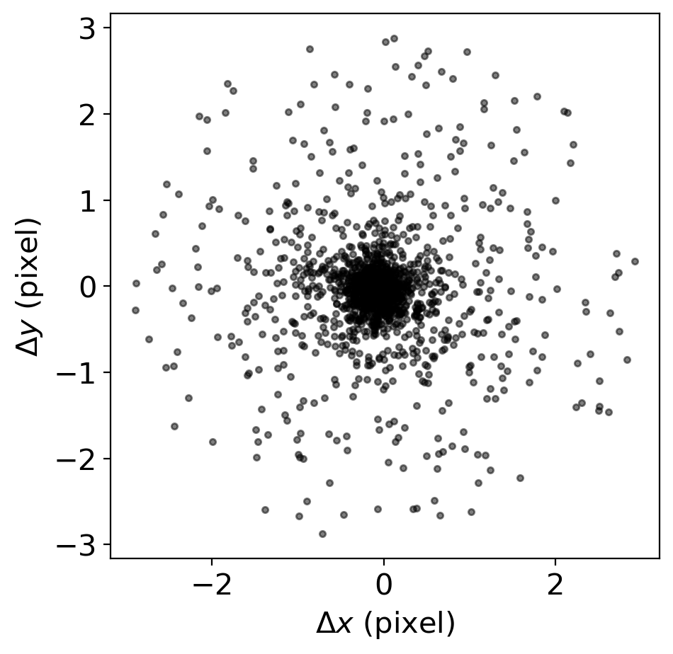
# let's check how well the matching went by plotting the difference of positions of the stars
# if the rlim=3.0 is too large, then try smaller value and repeat the matching process
# rlim ~< FWHM is recommended
fig = plt.figure(figsize=(5,5))
ax = fig.add_subplot(111)
ax.plot(grtbl['x_fit_r']-grtbl['x_fit_g'], grtbl['y_fit_r']-grtbl['y_fit_g'], '.k', alpha=0.5)
ax.set_xlabel('$\Delta x$ (pixel)')
ax.set_ylabel('$\Delta y$ (pixel)')
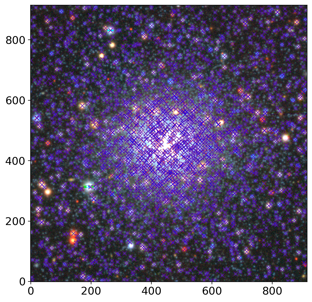
fig = plt.figure(figsize=(7,7))
ax = fig.add_subplot(111)
rgbimg = fits.getdata(DATADIR/'NGC2210.grz.rgb.fits')
ax.imshow(rgbimg, origin='lower')
ax.plot(grtbl['x_fit_r'], grtbl['y_fit_r'], 'xr', alpha=0.5)
ax.plot(grtbl['x_fit_g'], grtbl['y_fit_g'], 'xb', alpha=0.5)
<>:7: SyntaxWarning: invalid escape sequence '\D'
<>:8: SyntaxWarning: invalid escape sequence '\D'
<>:7: SyntaxWarning: invalid escape sequence '\D'
<>:8: SyntaxWarning: invalid escape sequence '\D'
/var/folders/c3/0f663kw90xldstvklyr5nq9c0000gn/T/ipykernel_6485/2619397371.py:7: SyntaxWarning: invalid escape sequence '\D'
  ax.set_xlabel('$\Delta x$ (pixel)')
/var/folders/c3/0f663kw90xldstvklyr5nq9c0000gn/T/ipykernel_6485/2619397371.py:8: SyntaxWarning: invalid escape sequence '\D'
  ax.set_ylabel('$\Delta y$ (pixel)')
[<matplotlib.lines.Line2D at 0x28abb49e0>]
7. Color-Magnitude Diagram#
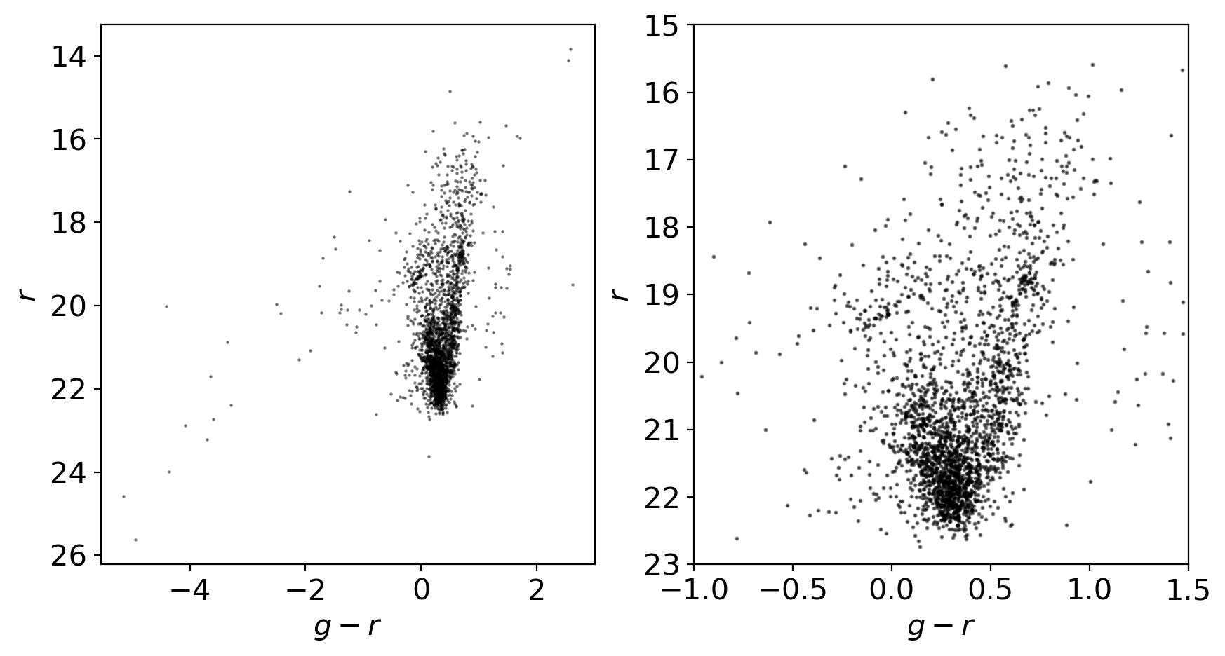
# then let's draw the color-magnitude diagram

def flux2mag(flux, zp=22.5): # the default zeropoint is set to 22.5 for the nanomaggy unit
    return -2.5*np.log10(flux) + zp

gmag = flux2mag(grtbl['flux_fit_g'])
rmag = flux2mag(grtbl['flux_fit_r'])

fig = plt.figure(figsize=(10,5))
ax = fig.add_subplot(121)
ax.scatter(gmag-rmag, rmag, marker='.', s=1.5, c='k', alpha=0.5)
ax.set_xlabel('$g-r$')
ax.set_ylabel('$r$')
ax.invert_yaxis()

# let's plot the color-magnitude diagram focusing on the non-outliers
ax2 = fig.add_subplot(122)
ax2.scatter(gmag-rmag, rmag, marker='.', s=5, c='k', alpha=0.5)
ax2.set_xlabel('$g-r$')
ax2.set_ylabel('$r$')
ax2.invert_yaxis()
ax2.set_xlim(-1, 1.5)
ax2.set_ylim(23, 15)
/var/folders/c3/0f663kw90xldstvklyr5nq9c0000gn/T/ipykernel_6485/3953004836.py:4: RuntimeWarning: invalid value encountered in log10
  return -2.5*np.log10(flux) + zp
(23.0, 15.0)
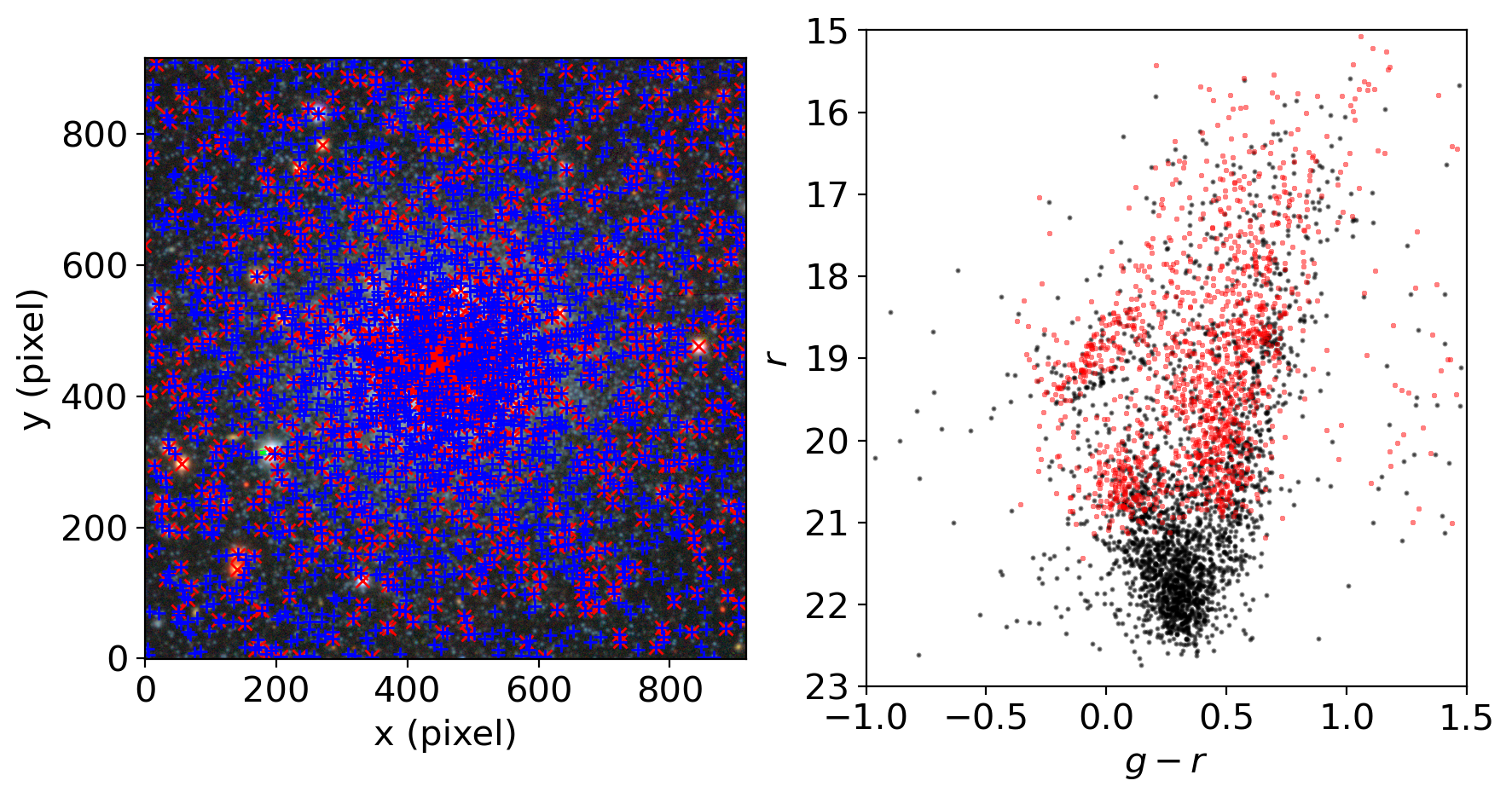
8. Comparison with the References#
# let's compare the color-magnitude diagram with the legacy survey catalog
vertices = ccd.wcs.celestial.calc_footprint()
ralo, rahi = vertices[:,0].min(), vertices[:,0].max()
declo, dechi = vertices[:,1].min(), vertices[:,1].max()

lgs_url = 'https://www.legacysurvey.org/viewer/ls-dr10/cat.fits?'
cat_bbox = f'ralo={ralo:.4f}&rahi={rahi:.4f}&declo={declo:.4f}&dechi={dechi:.4f}'

query_url = lgs_url + cat_bbox
cathdu = fits.open(query_url)

cat = Table(cathdu[1].data)
cat[:5].show_in_notebook()
# cat.show_in_notebook(display_length=10)
| idx | release | brickid | brickname | objid | brick_primary | maskbits | fitbits | type | ra | dec | ra_ivar | dec_ivar | bx | by | dchisq | ebv | mjd_min | mjd_max | ref_cat | ref_id | pmra | pmdec | parallax | pmra_ivar | pmdec_ivar | parallax_ivar | ref_epoch | gaia_phot_g_mean_mag | gaia_phot_g_mean_flux_over_error | gaia_phot_g_n_obs | gaia_phot_bp_mean_mag | gaia_phot_bp_mean_flux_over_error | gaia_phot_bp_n_obs | gaia_phot_rp_mean_mag | gaia_phot_rp_mean_flux_over_error | gaia_phot_rp_n_obs | gaia_phot_variable_flag | gaia_astrometric_excess_noise | gaia_astrometric_excess_noise_sig | gaia_astrometric_n_obs_al | gaia_astrometric_n_good_obs_al | gaia_astrometric_weight_al | gaia_duplicated_source | gaia_a_g_val | gaia_e_bp_min_rp_val | gaia_phot_bp_rp_excess_factor | gaia_astrometric_sigma5d_max | gaia_astrometric_params_solved | flux_g | flux_r | flux_i | flux_z | flux_w1 | flux_w2 | flux_w3 | flux_w4 | flux_ivar_g | flux_ivar_r | flux_ivar_i | flux_ivar_z | flux_ivar_w1 | flux_ivar_w2 | flux_ivar_w3 | flux_ivar_w4 | fiberflux_g | fiberflux_r | fiberflux_i | fiberflux_z | fibertotflux_g | fibertotflux_r | fibertotflux_i | fibertotflux_z | apflux_g | apflux_r | apflux_i | apflux_z | apflux_resid_g | apflux_resid_r | apflux_resid_i | apflux_resid_z | apflux_blobresid_g | apflux_blobresid_r | apflux_blobresid_i | apflux_blobresid_z | apflux_ivar_g | apflux_ivar_r | apflux_ivar_i | apflux_ivar_z | apflux_masked_g | apflux_masked_r | apflux_masked_i | apflux_masked_z | apflux_w1 | apflux_w2 | apflux_w3 | apflux_w4 | apflux_resid_w1 | apflux_resid_w2 | apflux_resid_w3 | apflux_resid_w4 | apflux_ivar_w1 | apflux_ivar_w2 | apflux_ivar_w3 | apflux_ivar_w4 | mw_transmission_g | mw_transmission_r | mw_transmission_i | mw_transmission_z | mw_transmission_w1 | mw_transmission_w2 | mw_transmission_w3 | mw_transmission_w4 | nobs_g | nobs_r | nobs_i | nobs_z | nobs_w1 | nobs_w2 | nobs_w3 | nobs_w4 | rchisq_g | rchisq_r | rchisq_i | rchisq_z | rchisq_w1 | rchisq_w2 | rchisq_w3 | rchisq_w4 | fracflux_g | fracflux_r | fracflux_i | fracflux_z | fracflux_w1 | fracflux_w2 | fracflux_w3 | fracflux_w4 | fracmasked_g | fracmasked_r | fracmasked_i | fracmasked_z | fracin_g | fracin_r | fracin_i | fracin_z | ngood_g | ngood_r | ngood_i | ngood_z | anymask_g | anymask_r | anymask_i | anymask_z | allmask_g | allmask_r | allmask_i | allmask_z | wisemask_w1 | wisemask_w2 | psfsize_g | psfsize_r | psfsize_i | psfsize_z | psfdepth_g | psfdepth_r | psfdepth_i | psfdepth_z | galdepth_g | galdepth_r | galdepth_i | galdepth_z | nea_g | nea_r | nea_i | nea_z | blob_nea_g | blob_nea_r | blob_nea_i | blob_nea_z | psfdepth_w1 | psfdepth_w2 | psfdepth_w3 | psfdepth_w4 | wise_coadd_id | wise_x | wise_y | lc_flux_w1 | lc_flux_w2 | lc_flux_ivar_w1 | lc_flux_ivar_w2 | lc_nobs_w1 | lc_nobs_w2 | lc_fracflux_w1 | lc_fracflux_w2 | lc_rchisq_w1 | lc_rchisq_w2 | lc_mjd_w1 | lc_mjd_w2 | lc_epoch_index_w1 | lc_epoch_index_w2 | sersic | sersic_ivar | shape_r | shape_r_ivar | shape_e1 | shape_e1_ivar | shape_e2 | shape_e2_ivar |
|---|---|---|---|---|---|---|---|---|---|---|---|---|---|---|---|---|---|---|---|---|---|---|---|---|---|---|---|---|---|---|---|---|---|---|---|---|---|---|---|---|---|---|---|---|---|---|---|---|---|---|---|---|---|---|---|---|---|---|---|---|---|---|---|---|---|---|---|---|---|---|---|---|---|---|---|---|---|---|---|---|---|---|---|---|---|---|---|---|---|---|---|---|---|---|---|---|---|---|---|---|---|---|---|---|---|---|---|---|---|---|---|---|---|---|---|---|---|---|---|---|---|---|---|---|---|---|---|---|---|---|---|---|---|---|---|---|---|---|---|---|---|---|---|---|---|---|---|---|---|---|---|---|---|---|---|---|---|---|---|---|---|---|---|---|---|---|---|---|---|---|---|---|---|---|---|---|---|---|---|---|---|---|---|---|---|---|---|---|---|---|---|---|---|---|---|---|---|---|---|---|---|---|---|---|---|---|---|
| 0 | 10000 | 21606 | 0928m692 | 3632 | True | 8192 | 129 | PSF | 92.78757007578037 | -69.12959365210126 | 62271860000000.0 | 99642075000000.0 | 1867.9648 | 3453.933 | 143652.3 .. 0.0 | 0.072651625 | 57283.31326590667 | 59268.07856435075 | GE | 5279742686399885312 | 1.3109009 | 1.4812818 | -0.070761435 | 2.3821611 | 5.770945 | 5.594181 | 2016.0 | 20.15112 | 192.3021 | 270 | 20.435118 | 18.27049 | 0 | 19.89739 | 12.570855 | 0 | False | 1.1294675 | 0.91282725 | 0 | 0 | 0.0 | False | 0.0 | 0.0 | 1.0900487 | 0.91672444 | 31 | 8.298511 | 8.945159 | 8.487956 | 8.432867 | 0.0 | 0.0 | 0.0 | 0.0 | 877.3331 | 718.1057 | 268.16235 | 90.84242 | 0.0 | 0.0 | 0.0 | 0.0 | 6.4651184 | 6.968902 | 6.6127095 | 6.569791 | 6.4646473 | 6.9683943 | 6.612228 | 6.569312 | 2.498601 .. 18.798218 | 3.2165787 .. 27.84321 | 2.270678 .. 25.20499 | 2.5010936 .. 27.251497 | -0.094051026 .. 6.24606 | -0.1272347 .. 11.613896 | -0.034183294 .. 8.227281 | -0.013881785 .. 9.485866 | -0.094051026 .. 6.24606 | -0.1272347 .. 11.613896 | -0.034183294 .. 8.227281 | -0.013881785 .. 9.485866 | 4302.66 .. 26.097149 | 2988.5078 .. 31.565092 | 1799.0396 .. 9.936828 | 550.3695 .. 2.77558 | 0.0 .. 0.0 | 0.0 .. 0.0 | 0.0 .. 0.0 | 0.0 .. 0.0 | 0.47616625 .. 2.2627623 | 0.34674054 .. 4.482998 | -1.2738854 .. -13.678328 | -1.0870681 .. -34.920433 | 0.46386555 .. 2.095589 | 0.34032154 .. 4.3984013 | -1.2854753 .. -13.803032 | -1.0955067 .. -35.15571 | 89.92067 .. 7.042809 | 21.144802 .. 1.5757307 | 0.3320874 .. 0.024630265 | 0.012552651 .. 0.0009306426 | 0.8064902 | 0.8651346 | 0.8989498 | 0.9221627 | 0.98776317 | 0.99246716 | 0.99838865 | 0.99939126 | 4 | 3 | 4 | 6 | 0 | 0 | 0 | 0 | 1.9490697 | 2.6909757 | 1.0727901 | 1.0382285 | 0.0 | 0.0 | 0.0 | 0.0 | 0.0008358622 | 0.0004906396 | 0.0030949514 | 0.0022943572 | 0.0 | 0.0 | 0.0 | 0.0 | 0.0054039187 | 0.0 | 0.00028888456 | 0.17291327 | 0.9999999 | 1.0000001 | 1.0 | 1.0 | 4 | 3 | 4 | 5 | 0 | 0 | 0 | 2048 | 0 | 0 | 0 | 0 | 0 | 0 | 1.423446 | 1.262223 | 1.523291 | 1.4677155 | 2335.5513 | 1391.1311 | 308.9544 | 97.81459 | 1479.8228 | 810.94653 | 198.52147 | 59.83889 | 4.56928 | 3.5420256 | 5.308711 | 4.830164 | 4.56936 | 3.5420852 | 5.3087926 | 4.0728116 | 0.0 | 0.0 | 0.0 | 0.0 | 0.0 | 0.0 | 0.0 .. 0.0 | 0.0 .. 0.0 | 0.0 .. 0.0 | 0.0 .. 0.0 | 0 .. 0 | 0 .. 0 | 0.0 .. 0.0 | 0.0 .. 0.0 | 0.0 .. 0.0 | 0.0 .. 0.0 | 0.0 .. 0.0 | 0.0 .. 0.0 | 0 .. 16 | 0 .. 16 | 0.0 | 0.0 | 0.0 | 0.0 | 0.0 | 0.0 | 0.0 | 0.0 | |
| 1 | 10000 | 21606 | 0928m692 | 3638 | True | 8192 | 129 | PSF | 92.78808919227178 | -69.12818970307045 | 31441444000000.0 | 57867800000000.0 | 1865.428 | 3473.2246 | 74006.31 .. 0.0 | 0.07256889 | 57283.31326590667 | 59268.07856435075 | GE | 5279742755130206336 | 2.680022 | 2.4693081 | 0.6905479 | 1.4555007 | 3.0879586 | 3.2713585 | 2016.0 | 20.50525 | 166.3184 | 279 | 21.08072 | 9.514463 | 0 | 20.037846 | 11.650101 | 0 | False | 0.7970623 | 0.24483252 | 0 | 0 | 0.0 | False | 0.0 | 0.0 | 1.0742582 | 1.1786243 | 95 | 4.264763 | 7.3260207 | 8.670622 | 9.5797825 | 0.0 | 0.0 | 0.0 | 0.0 | 212.29167 | 783.91205 | 264.03497 | 89.63854 | 0.0 | 0.0 | 0.0 | 0.0 | 3.3178408 | 5.699395 | 6.745449 | 7.452745 | 3.315516 | 5.6954017 | 6.740723 | 7.447523 | 1.3301907 .. 18.185356 | 2.6378582 .. 26.679947 | 2.2484665 .. 24.360357 | 2.7981932 .. 25.01609 | -0.10030402 .. 3.5931304 | -0.11436806 .. 8.013494 | -0.10821519 .. 4.957432 | -0.06148577 .. 4.714269 | -0.10030402 .. 3.5931304 | -0.11436806 .. 8.013494 | -0.10821519 .. 4.957432 | -0.06148577 .. 4.714269 | 927.5121 .. 21.609037 | 3344.3213 .. 31.58236 | 1766.0658 .. 10.62638 | 545.5569 .. 2.8899465 | 0.0 .. 0.0 | 0.0 .. 0.0 | 0.0 .. 0.0 | 0.0 .. 0.0 | 0.8132416 .. 4.6910753 | 0.7068993 .. 6.130646 | -2.7616856 .. -20.86119 | -0.3840622 .. -17.733297 | 0.7977932 .. 4.1131463 | 0.6985612 .. 5.8887625 | -2.7767415 .. -21.121397 | -0.40319905 .. -18.037237 | 87.94504 .. 6.904517 | 20.665148 .. 1.5657216 | 0.3306132 .. 0.024638768 | 0.0126051605 .. 0.0009347549 | 0.8066877 | 0.86527735 | 0.8990589 | 0.9222478 | 0.98777705 | 0.9924757 | 0.9983905 | 0.999392 | 4 | 3 | 4 | 6 | 0 | 0 | 0 | 0 | 1.0934112 | 3.0050054 | 1.7860744 | 0.8481531 | 0.0 | 0.0 | 0.0 | 0.0 | 0.0028263621 | 0.0011597461 | 0.0034827534 | 0.0021375008 | 0.0 | 0.0 | 0.0 | 0.0 | 0.22418965 | 0.0 | 6.584817e-07 | 0.18844916 | 0.99918 | 1.0 | 1.0 | 1.0 | 3 | 3 | 4 | 5 | 2048 | 0 | 0 | 2048 | 0 | 0 | 0 | 0 | 0 | 0 | 1.423446 | 1.262223 | 1.523291 | 1.4677155 | 273.65677 | 1391.1311 | 308.9544 | 97.81459 | 163.1253 | 810.94653 | 198.52147 | 59.83889 | 4.5589733 | 3.5416598 | 5.308278 | 4.829716 | 0.53446114 | 3.5417206 | 5.3083606 | 4.0724344 | 0.0 | 0.0 | 0.0 | 0.0 | 0.0 | 0.0 | 0.0 .. 0.0 | 0.0 .. 0.0 | 0.0 .. 0.0 | 0.0 .. 0.0 | 0 .. 0 | 0 .. 0 | 0.0 .. 0.0 | 0.0 .. 0.0 | 0.0 .. 0.0 | 0.0 .. 0.0 | 0.0 .. 0.0 | 0.0 .. 0.0 | 0 .. 16 | 0 .. 16 | 0.0 | 0.0 | 0.0 | 0.0 | 0.0 | 0.0 | 0.0 | 0.0 | |
| 2 | 10000 | 21606 | 0928m692 | 3641 | True | 8192 | 129 | PSF | 92.78849191182563 | -69.13793761028107 | 47808930000000.0 | 73617224000000.0 | 1863.428 | 3339.2837 | 124841.4 .. 0.0 | 0.07312917 | 57283.31326590667 | 59268.07856435075 | GE | 5279742686416209152 | 0.2521983 | 1.4458102 | -0.016146168 | 2.183477 | 2.5972373 | 4.1903563 | 2016.0 | 20.36864 | 175.94759 | 275 | 20.509983 | 8.335049 | 0 | 19.746296 | 15.887417 | 0 | False | 0.0 | 0.0 | 0 | 0 | 0.0 | False | 0.0 | 0.0 | 1.383404 | 1.0020562 | 31 | 6.367055 | 8.38598 | 9.369133 | 8.916471 | 0.0 | 0.0 | 0.0 | 0.0 | 1034.6625 | 752.45465 | 265.2095 | 84.30954 | 0.0 | 0.0 | 0.0 | 0.0 | 4.950536 | 6.5202966 | 7.284722 | 6.9327664 | 4.9503098 | 6.5199995 | 7.28439 | 6.9324503 | 1.7929345 .. 83.36924 | 2.8661578 .. 136.46315 | 2.3365793 .. 152.70065 | 2.6167917 .. 169.7976 | -0.1991595 .. 8.943009 | -0.26675004 .. 15.530283 | -0.17375015 .. 10.050449 | -0.16860354 .. 12.066279 | -0.1991595 .. 8.943009 | -0.26675004 .. 15.530283 | -0.17375015 .. 10.050449 | -0.16860354 .. 12.066279 | 5254.3286 .. 51.78501 | 3218.978 .. 26.604462 | 1767.5148 .. 9.691271 | 486.22397 .. 2.5952268 | 0.0 .. 0.0 | 0.0 .. 0.0 | 0.0 .. 0.0 | 0.0 .. 0.0 | 7.5557785 .. 55.45823 | 4.264436 .. 33.605732 | -3.201238 .. -26.795685 | -11.259108 .. -30.212961 | 7.5557785 .. 55.45823 | 4.264436 .. 33.605732 | -3.201238 .. -26.795685 | -11.259108 .. -30.212961 | 40.17313 .. 4.201287 | 15.625595 .. 1.3296257 | 0.33043286 .. 0.024583036 | 0.012395947 .. 0.000922885 | 0.8053509 | 0.8643112 | 0.89832056 | 0.9216716 | 0.98768324 | 0.9924178 | 0.9983781 | 0.99938726 | 4 | 3 | 4 | 6 | 0 | 0 | 0 | 0 | 6.798843 | 9.814107 | 3.5114033 | 1.0228102 | 0.0 | 0.0 | 0.0 | 0.0 | 0.014635966 | 0.013884812 | 0.04122043 | 0.038656782 | 0.0 | 0.0 | 0.0 | 0.0 | 0.0 | 0.0 | 0.00093237247 | 0.24141891 | 0.99999994 | 1.0 | 0.9999999 | 1.0 | 4 | 3 | 4 | 5 | 0 | 0 | 0 | 2048 | 0 | 0 | 0 | 0 | 0 | 0 | 1.423446 | 1.262223 | 1.523291 | 1.4677155 | 2335.5513 | 1391.1311 | 308.9544 | 97.81459 | 1479.8228 | 810.94653 | 198.52147 | 59.83889 | 4.5753913 | 3.5604668 | 5.2925844 | 4.8279014 | 4.57547 | 3.5605273 | 5.2926683 | 4.070905 | 0.0 | 0.0 | 0.0 | 0.0 | 0.0 | 0.0 | 0.0 .. 0.0 | 0.0 .. 0.0 | 0.0 .. 0.0 | 0.0 .. 0.0 | 0 .. 0 | 0 .. 0 | 0.0 .. 0.0 | 0.0 .. 0.0 | 0.0 .. 0.0 | 0.0 .. 0.0 | 0.0 .. 0.0 | 0.0 .. 0.0 | 0 .. 16 | 0 .. 16 | 0.0 | 0.0 | 0.0 | 0.0 | 0.0 | 0.0 | 0.0 | 0.0 | |
| 3 | 10000 | 21606 | 0928m692 | 3644 | True | 8192 | 129 | PSF | 92.78882908793277 | -69.14851665017197 | 13858959000000.0 | 16943370000000.0 | 1861.7478 | 3193.9226 | 43837.08 .. 0.0 | 0.07379439 | 57283.31326590667 | 59268.07856435075 | GE | 5279695751008126976 | 1.3003335 | 0.5740968 | -0.74506813 | 0.7130624 | 1.3627695 | 0.9639698 | 2016.0 | 20.817247 | 99.491905 | 172 | 21.026443 | 9.564173 | 0 | 20.640682 | 7.5729084 | 0 | False | 0.0 | 0.0 | 0 | 0 | 0.0 | False | 0.0 | 0.0 | 1.0933896 | 1.7364924 | 95 | 4.3015213 | 4.6295485 | 4.4563084 | 4.3970356 | 0.0 | 0.0 | 0.0 | 0.0 | 926.8981 | 926.74927 | 251.75075 | 94.46215 | 0.0 | 0.0 | 0.0 | 0.0 | 3.349544 | 3.6049752 | 3.4700751 | 3.4239202 | 3.3495069 | 3.6049352 | 3.4700365 | 3.423882 | 1.3143821 .. 31.190805 | 1.6728723 .. 54.66553 | 1.1416255 .. 58.541225 | 1.3034669 .. 67.23993 | -0.032942876 .. 3.879783 | -0.046171136 .. 9.670687 | -0.032774374 .. 7.0183578 | -0.012071089 .. 11.460372 | -0.032942876 .. 3.879783 | -0.046171136 .. 9.670687 | -0.032774374 .. 7.0183578 | -0.012071089 .. 11.460372 | 2076.3816 .. 6.543746 | 3999.7795 .. 29.48291 | 1733.6534 .. 9.708909 | 577.8104 .. 2.4030948 | 0.0 .. 0.09631865 | 0.0 .. 0.0 | 0.0 .. 0.0 | 0.0 .. 0.0 | 2.2776866 .. 42.42142 | 1.4591917 .. 27.440006 | -4.0022893 .. 4.625561 | -4.2769136 .. 41.47543 | 2.2776866 .. 42.42142 | 1.4591917 .. 27.440006 | -4.0022893 .. 4.625561 | -4.2769136 .. 41.47543 | 64.83757 .. 4.7248554 | 18.852259 .. 1.3727484 | 0.32796517 .. 0.024412338 | 0.012417219 .. 0.0009265517 | 0.80376655 | 0.8631655 | 0.8974448 | 0.9209881 | 0.9875719 | 0.99234915 | 0.9983633 | 0.99938166 | 4 | 3 | 3 | 6 | 0 | 0 | 0 | 0 | 0.8198578 | 1.6131167 | 1.0032206 | 0.7844196 | 0.0 | 0.0 | 0.0 | 0.0 | 0.007130165 | 0.007151729 | 0.03338568 | 0.023207674 | 0.0 | 0.0 | 0.0 | 0.0 | 0.20330389 | 0.00012891984 | 0.00094950583 | 0.19042052 | 0.99988294 | 0.97003776 | 0.8094458 | 0.99981916 | 4 | 3 | 3 | 5 | 0 | 0 | 0 | 2048 | 0 | 0 | 0 | 0 | 0 | 0 | 1.423446 | 1.262223 | 1.5549465 | 1.4677155 | 2335.5513 | 1391.1311 | 266.39575 | 97.81459 | 1479.8228 | 810.94653 | 173.5426 | 59.83889 | 4.575948 | 3.5502062 | 5.2382827 | 4.8365474 | 4.5760922 | 3.5801198 | 5.4093647 | 4.079353 | 0.0 | 0.0 | 0.0 | 0.0 | 0.0 | 0.0 | 0.0 .. 0.0 | 0.0 .. 0.0 | 0.0 .. 0.0 | 0.0 .. 0.0 | 0 .. 0 | 0 .. 0 | 0.0 .. 0.0 | 0.0 .. 0.0 | 0.0 .. 0.0 | 0.0 .. 0.0 | 0.0 .. 0.0 | 0.0 .. 0.0 | 0 .. 16 | 0 .. 16 | 0.0 | 0.0 | 0.0 | 0.0 | 0.0 | 0.0 | 0.0 | 0.0 | |
| 4 | 10000 | 21606 | 0928m692 | 3647 | True | 8192 | 129 | PSF | 92.78952269793871 | -69.1387958994378 | 14409476000000.0 | 28886644000000.0 | 1858.3817 | 3327.4915 | 59808.633 .. 0.0 | 0.07317518 | 57283.31326590667 | 59268.07856435075 | GE | 5279742686416267392 | -0.8915288 | 0.40552515 | 0.1306394 | 0.5406098 | 0.85731494 | 1.7357312 | 2016.0 | 20.747555 | 114.866806 | 162 | 21.65588 | 7.766733 | 0 | 20.397083 | 5.1676884 | 0 | False | 0.0 | 1.6806109e-15 | 0 | 0 | 0.0 | False | 0.0 | 0.0 | 0.8954515 | 1.9916974 | 95 | 3.468565 | 5.590245 | 6.6708765 | 7.419922 | 0.0 | 0.0 | 0.0 | 0.0 | 1355.5065 | 872.0004 | 274.76895 | 73.05946 | 0.0 | 0.0 | 0.0 | 0.0 | 2.693272 | 4.340715 | 5.179804 | 5.761423 | 2.6937149 | 4.3414283 | 5.1806555 | 5.76237 | 1.0480822 .. 73.521286 | 2.0099716 .. 127.48353 | 1.782606 .. 145.57591 | 2.078548 .. 163.38074 | -0.041219242 .. 9.795995 | -0.07765031 .. 16.660069 | -0.039027747 .. 11.232489 | -0.013793198 .. 13.646062 | -0.041219242 .. 9.795995 | -0.07765031 .. 16.660069 | -0.039027747 .. 11.232489 | -0.013793198 .. 13.646062 | 7059.858 .. 53.469273 | 3730.3472 .. 26.958393 | 1835.2968 .. 10.0860815 | 482.82944 .. 2.678223 | 0.0 .. 0.0 | 0.0 .. 0.0 | 0.0 .. 0.0 | 0.0 .. 0.0 | 6.2135167 .. 59.95758 | 3.531377 .. 35.15216 | -0.92712647 .. -27.9808 | -7.43345 .. -41.60498 | 6.2135167 .. 59.95758 | 3.531377 .. 35.15216 | -0.92712647 .. -27.9808 | -7.43345 .. -41.60498 | 40.100945 .. 4.040845 | 15.733147 .. 1.3151103 | 0.33136323 .. 0.024576368 | 0.01244733 .. 0.0009234766 | 0.8052412 | 0.8642319 | 0.89826 | 0.92162436 | 0.98767555 | 0.9924131 | 0.998377 | 0.9993869 | 4 | 3 | 4 | 6 | 0 | 0 | 0 | 0 | 1.5222948 | 1.752035 | 1.1288128 | 0.6500207 | 0.0 | 0.0 | 0.0 | 0.0 | 0.023820776 | 0.019542458 | 0.06313007 | 0.045995627 | 0.0 | 0.0 | 0.0 | 0.0 | 4.8863744e-09 | 0.0 | 6.8382506e-05 | 0.33307713 | 1.0 | 0.9999999 | 0.99999994 | 0.99999994 | 4 | 3 | 4 | 4 | 0 | 0 | 0 | 2048 | 0 | 0 | 0 | 0 | 0 | 0 | 1.423446 | 1.262223 | 1.523291 | 1.4677155 | 2335.5513 | 1391.1311 | 308.9544 | 77.65208 | 1479.8228 | 810.94653 | 198.52147 | 49.08919 | 4.5763483 | 3.5592587 | 5.2900586 | 4.8293376 | 4.5764275 | 3.55932 | 5.290142 | 3.2327316 | 0.0 | 0.0 | 0.0 | 0.0 | 0.0 | 0.0 | 0.0 .. 0.0 | 0.0 .. 0.0 | 0.0 .. 0.0 | 0.0 .. 0.0 | 0 .. 0 | 0 .. 0 | 0.0 .. 0.0 | 0.0 .. 0.0 | 0.0 .. 0.0 | 0.0 .. 0.0 | 0.0 .. 0.0 | 0.0 .. 0.0 | 0 .. 16 | 0 .. 16 | 0.0 | 0.0 | 0.0 | 0.0 | 0.0 | 0.0 | 0.0 | 0.0 |
gcat = flux2mag(cat['flux_g']) # nanomaggy to magnitude
rcat = flux2mag(cat['flux_r'])

xcat, ycat = ccd.wcs.celestial.all_world2pix(cat['ra'], cat['dec'], 0)
cat['x'] = xcat
cat['y'] = ycat

fig = plt.figure(figsize=(10,5))
ax = fig.add_subplot(121)
ax.imshow(rgbimg, origin='lower')
ax.plot(xcat, ycat, 'xr')
ax.plot(grtbl['x_fit_g'], grtbl['y_fit_g'], '+b')
ax.set_xlabel('x (pixel)')
ax.set_ylabel('y (pixel)')
ax.set_xlim(0, len(rgbimg[0]))

ax2 = fig.add_subplot(122)
ax2.scatter(gmag-rmag, rmag, marker='.', s=5, c='k', alpha=0.5)
ax2.scatter(gcat-rcat, rcat, marker='+', s=5, c='r', alpha=0.5)
ax2.set_xlabel('$g-r$')
ax2.set_ylabel('$r$')
ax2.invert_yaxis()
ax2.set_xlim(-1, 1.5)
ax2.set_ylim(23, 15)
/var/folders/c3/0f663kw90xldstvklyr5nq9c0000gn/T/ipykernel_6485/3953004836.py:4: RuntimeWarning: invalid value encountered in log10
  return -2.5*np.log10(flux) + zp
(23.0, 15.0)
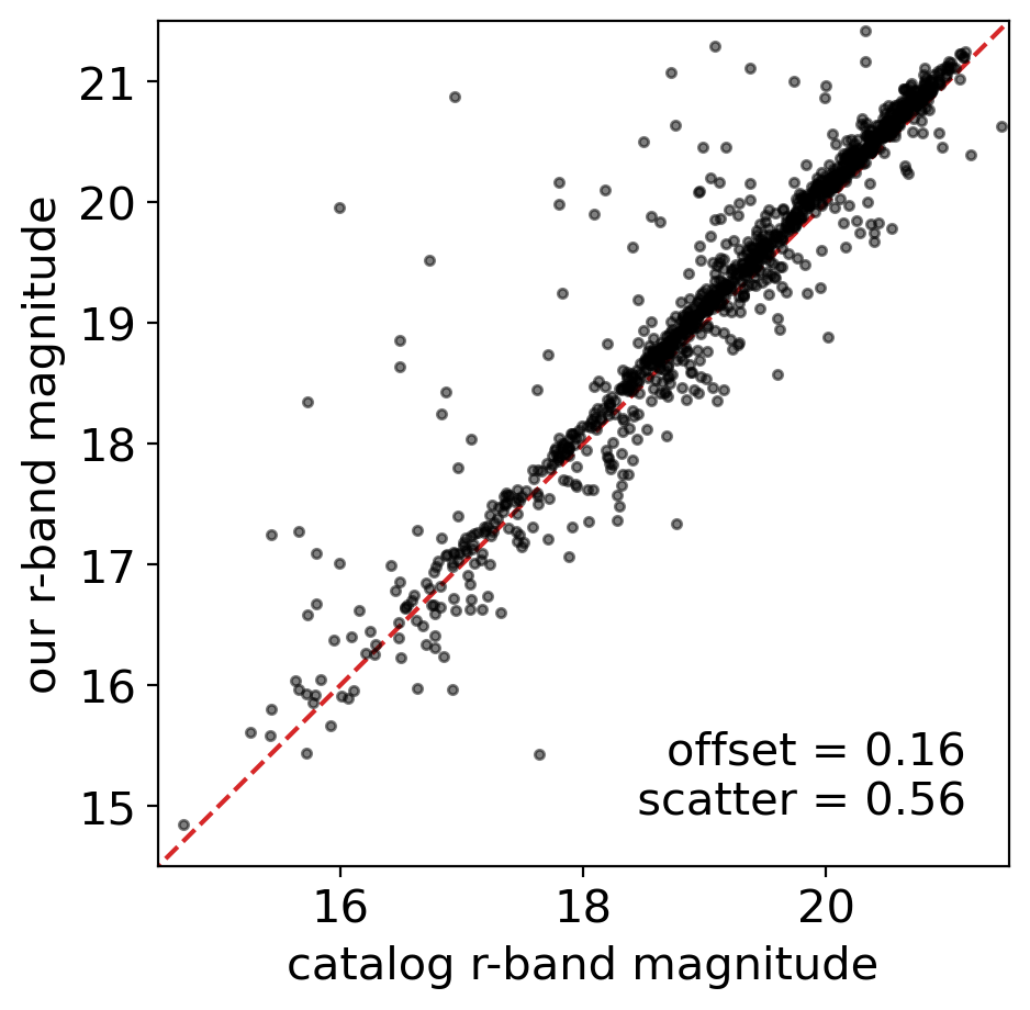
# let's match the stars in the catalog with the stars of our photometry
cmtbl_r = match_stars(rtbl, cat, ['our', 'cat'], refcard=['x_fit', 'y_fit'],
                    objcard=['x', 'y', 'flux_r'], rlim=rlim)
# and compare the magnitude
fig = plt.figure(figsize=(5,5))
ax = fig.add_subplot(111)
crmag = flux2mag(cmtbl_r['flux_r']) # catalog r-band magnitude
ormag = flux2mag(cmtbl_r['flux_fit']) # our r-band magnitude
ax.plot(crmag, ormag, '.k', alpha=0.5)
ax.set_ylim([14.5, 21.5])
ax.set_xlim([14.5, 21.5])
ax.plot([14, 22], [14, 22], ls='--', c='tab:red', zorder=0)
ax.set_xlabel('catalog r-band magnitude')
ax.set_ylabel('our r-band magnitude')

diff = ormag - crmag
offset, scatter = np.nanmean(diff), np.nanstd(diff)

ax.text(0.95, 0.05, f'offset = {offset:.2f}\n scatter = {scatter:.2f}',
        transform=ax.transAxes, va='bottom', ha='right')
/var/folders/c3/0f663kw90xldstvklyr5nq9c0000gn/T/ipykernel_6485/3953004836.py:4: RuntimeWarning: invalid value encountered in log10
  return -2.5*np.log10(flux) + zp
Text(0.95, 0.05, 'offset = 0.16\n scatter = 0.56')
# doing the same thing in gz-band
cmtbl_g = match_stars(gtbl, cat, ['our', 'cat'], refcard=['x_fit', 'y_fit'],
                      objcard=['x', 'y', 'flux_g'], rlim=rlim)
cmtbl_z = match_stars(ztbl, cat, ['our', 'cat'], refcard=['x_fit', 'y_fit'],
                      objcard=['x', 'y', 'flux_z'], rlim=rlim)
fig, axes = plt.subplots(1, 3, figsize=(15,5))
cgmag = flux2mag(cmtbl_g['flux_g']) # catalog g-band magnitude
ogmag = flux2mag(cmtbl_g['flux_fit']) # our g-band magnitude
czmag = flux2mag(cmtbl_z['flux_z']) # catalog z-band magnitude
ozmag = flux2mag(cmtbl_z['flux_fit']) # our z-band magnitude
for ax, cmag, omag, band in zip(axes, [cgmag, crmag, czmag],
                                [ogmag, ormag, ozmag], ['g', 'r', 'z']):
    ax.plot(cmag, omag, '.k', alpha=0.5)
    ax.set_ylim([14.5, 22])
    ax.set_xlim([14.5, 22])
    ax.plot([14, 22], [14, 22], ls='--', c='tab:red', zorder=0)
    ax.set_xlabel(f'catalog {band}-band magnitude')
    ax.set_ylabel(f'our {band}-band magnitude')

    diff = omag - cmag
    offset, scatter = np.nanmean(diff), np.nanstd(diff)

    ax.text(0.95, 0.05, f'offset = {offset:.2f}\n scatter = {scatter:.2f}',
            transform=ax.transAxes, va='bottom', ha='right')
/var/folders/c3/0f663kw90xldstvklyr5nq9c0000gn/T/ipykernel_6485/3953004836.py:4: RuntimeWarning: invalid value encountered in log10
  return -2.5*np.log10(flux) + zp
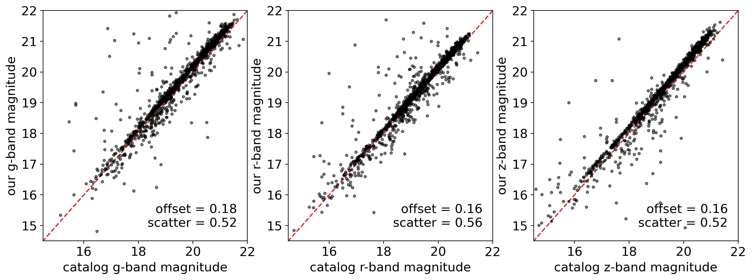
There are systematic offsets between cataloged magnitude and our PSF magnitude, for each band. What made these offsets? Who derived more correct result? There are many possible reasons of the offsets one can think of:
Difference in aperture correction process between our method and
Tractor, which is the tool for extracting PSF magnitude in DESI Legacy Survey catalog.Difference in PSF model - only a percent level error in PSF model can 10~100% errors of the faint star near the bright stars. The systematic offset in PSF model can derive the systematic offsets in the magnitude.
Difference in the background subtraction
And many more -
One possible way to resolve the cause of the offset is compare the PSF photometry at the un-crowded field, to find out how the crowding affects the resulting magnitudes. Another way is simulate a star inside the image and repeat the photometry over, and compare the input with the magnitudes from the PSF photometry, which is called the artificial star test.
I will leave this task to the reader.
To compare with another reference with the \(BV\) magnitude, we need a transformation relation of our \(gr\) magnitude into \(BV\) magnitude.
Transformation from DECam \(griz\) to Johnson-Cousins (\(UBV R_C I_C\)) system
def Bmag(gmag, rmag):
    B = np.zeros_like(gmag)
    gmr = gmag - rmag
    blu = (gmr > -0.5) & (gmr <= 0.2)
    grn = (gmr > 0.2) & (gmr <= 0.7)
    red = (gmr > 0.7) & (gmr <= 1.8)
    B[blu] = gmag[blu] + 0.371*gmr[blu] + 0.197
    B[grn] = gmag[grn] + 0.542*gmr[grn] + 0.141
    B[red] = gmag[red] + 0.454*gmr[red] + 0.200
    return B

def Vmag(gmag, rmag):
    V = np.zeros_like(gmag)
    gmr = gmag - rmag
    blu = (gmr > -0.5) & (gmr <= 0.2)
    grn = (gmr > 0.2) & (gmr <= 0.7)
    red = (gmr > 0.7) & (gmr <= 1.8)
    V[blu] = gmag[blu] - 0.465*gmr[blu] - 0.020
    V[grn] = gmag[grn] - 0.496*gmr[grn] - 0.015
    V[red] = gmag[red] - 0.445*gmr[red] - 0.062
    return V

B, V = Bmag(gmag, rmag), Vmag(gmag, rmag)

# let's compare the color-magnitude diagram of ours to the reference
# reference: Peter Stetson's stellar standards and software - Homogeneous photometry
# one can download the data from https://www.cadc.hia.nrc.gc.ca/en/community/STETSON/homogeneous/

# read the reference data
reftbl = Table.read(DATADIR/'stetson'/'NGC2210.dat', format='ascii.fixed_width_two_line')
# plot the color-magnitude diagram
fig = plt.figure(figsize=(7,7))
ax = fig.add_subplot(111)
ax.scatter(reftbl['B']-reftbl['V'], reftbl['V'], marker='.', s=1, c='k', alpha=0.3, label='Stetson')
ax.scatter(B-V, V, marker='.', s=5, c='r', alpha=0.5, label='Our result')
ax.set_ylim([14.5, 22])
ax.set_xlim([-1, 2])
ax.set_xlabel('$B-V$')
ax.set_ylabel('$V$')
ax.invert_yaxis()
ax.legend(markerscale=5)
<matplotlib.legend.Legend at 0x176307f20>
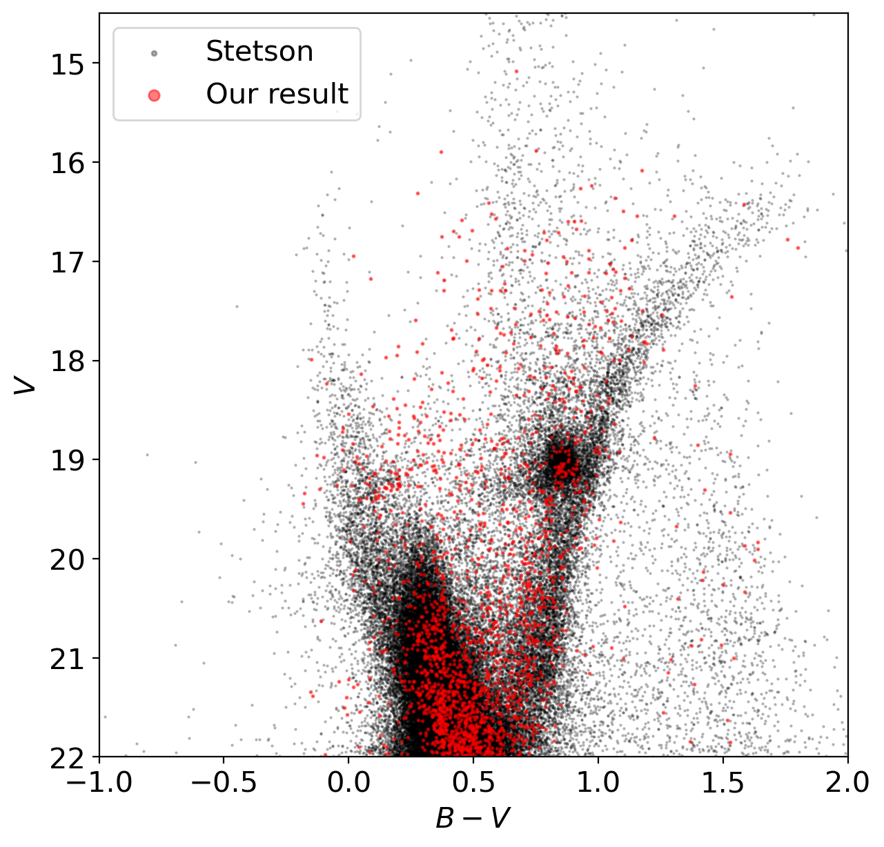
From the color-magnitude diagram we obtained, which properties of this system will you be able to find out?
Properties of stars inside this field
Properties of the globular cluster NGC 2210
Is our photometry reliable?
etc
Further Readings#
Stetson (1987PASP…99…191S), DAOPHOT: A Computer Program for Crowded-Field Stellar Photometry
Seminal paper about how to find stars and do photometry from a CCD image over crowded field
Anderson & King (2000PASP…112.1360A), Toward High-Precision Astrometry with WFPC2. I. Deriving an Accurate Point-Spread Function
This work describes how the effective point-spread function is estimated.
Stetson et al. (2019MNRAS.485.3042S), Homogeneous photometry - VII. Globular clusters in the Gaia era
Modern homogeneous photometry given by Peter Stetson, especially for the globular clusters, by conducting the PSF photometry.
Baumgardt et al. (2023MNRAS.521.3991B), Evidence for a bottom-light initial mass function in massive star clusters
This reference may gave you some idea about how member stars in a cluster can be identified.